Fitur Pembuatan Gambar AI Gratitude, dibangun dalam waktu rekaman dengan bantuan Gemini di Android Studio
Membuka Efisiensi Baru dengan Gemini di Android Studio
Tim terima kasih memutuskan untuk mencoba Gemini di Android Studio, seorang asisten AI yang mendukung pengembang di semua tahap pengembangan, membantu mereka menjadi lebih produktif. Pengembang dapat mengajukan pertanyaan Gemini dan menerima solusi sadar-konteks berdasarkan kode mereka. Divij Gupta, pengembang senior Android dengan rasa terima kasih, berbagi bahwa tim terima kasih perlu mengetahui apakah mungkin untuk menyuntikkan objek apa pun ke dalam kelas objek Kotlin menggunakan Hilt. Gemini menyarankan menggunakan titik masuk untuk mengakses dependensi di kelas di mana injeksi standar tidak mungkin, yang membantu menyelesaikan “masalah rumit mereka,” menurut Divij.
Gemini menghilangkan kebutuhan untuk mencari dokumentasi Android juga, memungkinkan tim terima kasih untuk belajar dan menerapkan pengetahuan mereka tanpa harus meninggalkan Android Studio. “Gemini menunjukkan kepada saya cara menggunakan CPU Android Studio dan profiler memori secara lebih efektif,” kenang Divij. “Saya juga belajar cara mengatur profil awal untuk mempercepat awal yang dingin.”
Mengidentifikasi hambatan kinerja menjadi lebih mudah. Saat menganalisis kode tim terima kasih, Gemini menyarankan untuk menggunakan CollectAstateWithLifeCycle alih-alih collectasstate Untuk mengumpulkan aliran di komposable, yang membantu aplikasi menangani peristiwa siklus hidup lebih efektif dan meningkatkan kinerja secara keseluruhan. Gemini juga menganalisis laporan crash aplikasi di Wawasan kualitas aplikasi Panel dan memberikan panduan tentang cara mengatasi setiap masalah, yang memungkinkan tim terima kasih untuk “mengidentifikasi akar penyebab lebih cepat, menangkap kasus tepi yang mungkin kami lewatkan, dan meningkatkan stabilitas aplikasi secara keseluruhan,” menurut Divij.
Bereksperimen dengan fitur baru menggunakan Gemini di Android Studio
Gemini di Android Studio membantu tim terima kasih secara signifikan meningkatkan kecepatan dan moral pengembangan mereka. “Siklus yang lebih cepat ini telah membuat tim merasa lebih produktif, termotivasi, dan bersemangat untuk terus berinovasi,” kata Divij. Pengembang dapat menghabiskan lebih banyak waktu untuk mengidentifikasi dan bereksperimen pada fitur -fitur baru, yang mengarah pada pengalaman baru yang inovatif.
Salah satu fitur yang dibangun pengembang dengan waktu ditemukan baru adalah fungsi pembuatan gambar untuk fitur papan visi aplikasi. Pengguna sekarang dapat mengunggah foto dengan prompt, dan kemudian menerima gambar yang dihasilkan AI yang mereka dapat langsung menjepit papan mereka. Tim dapat membangun UI menggunakan Gemini di Android Studio Menyusun pembuatan pratinjau -memungkinkan mereka untuk dengan cepat memvisualisasikan kode jetpack mereka dan membuat piksel-perfect ui yang dimaksudkan oleh desainer mereka.
Ke depan, tim terima kasih berharap untuk menggunakan Gemini untuk menerapkan lebih banyak peningkatan pada kodenya, termasuk mengoreksi gangguan, kebocoran memori, dan meningkatkan kinerja berdasarkan lebih banyak wawasan dari Gemini, yang selanjutnya akan meningkatkan pengalaman pengguna.
Posted by Mayuri Khinvasara Khabya – Developer Relations Engineer (LinkedIn and X)
Welcome to the second installment of our three-part series on media preloading with Media3. This series is designed to guide you through the process of building highly responsive, low-latency media experiences in your Android apps.
Part 1: Introducing Preloading with Media3 covered the fundamentals. We explored the distinction between PreloadConfiguration for simple playlists and the more powerful DefaultPreloadManager for dynamic user interfaces. You learned how to implement the basic API lifecycle: adding media with add(), retrieving a prepared MediaSource with getMediaSource(), managing priorities with setCurrentPlayingIndex() and invalidate(), and releasing resources with remove() and release().
Part 2 (This post): In this blog, we explore the advanced capabilities of the DefaultPreloadManager. We cover how to gain insights with PreloadManagerListener, implement production-ready best practices like sharing core components with ExoPlayer, and master the sliding window pattern to effectively manage memory.
Part 3: The final part of this series will dive into integrating PreloadManager with a persistent disk cache, enabling you to reduce data consumption with resource management and provide a seamless experience.
If you are new to preloading in Media3, we highly recommend reading Part 1 before proceeding. For those ready to move beyond the basics, let’s explore how to elevate your media playback implementation.
Listening in: Fetch analytics with PreloadManagerListener
When you want to launch a feature in production, as an app developer you also want to understand and capture the analytics behind it. How can you be certain that your preloading strategy is effective in a real-world environment? Answering this requires data on success rates, failures, and performance. The PreloadManagerListener interface is the primary mechanism for gathering this data.
The PreloadManagerListener provides two essential callbacks that offer critical insights into the preloading process and status.
onCompleted(MediaItem mediaItem): This callback is invoked upon the successful completion of a preload request, as defined by your TargetPreloadStatusControl.
onError(PreloadException error): This callback could be useful for debugging and monitoring. It is invoked when a preload fails, providing the associated exception.
You can register a listener with a single method call as shown in the following example code:
valpreloadManagerListener=object:PreloadManagerListener{
overridefunonCompleted(mediaItem:MediaItem){
// Log success for analytics. Log.d("PreloadAnalytics","Preload completed for $mediaItem")
}
overridefunonError(preloadError:PreloadException){
// Log the specific error for debugging and monitoring.Log.e("PreloadAnalytics","Preload error ",preloadError)
}
}
preloadManager.addListener(preloadManagerListener)
Extracting insights from the listener
These listener callbacks can be hooked to your analytics pipeline. By forwarding these events to your analytics engine, you can answer key questions like:
What is our preload success rate? (ratio of onCompleted events to total preload attempts)
Which CDNs or video formats exhibit the highest error rates? (By parsing the exceptions from onError)
What is our preload error rate? (ratio of onError events to total preload attempts)
This data could give you quantitative feedback on your preloading strategy, enabling A/B testing and data-driven improvements to your user experience. This data can further help you to intelligently finetune your preload durations and number of videos you want to preload as well as the buffers you allocate.
Beyond debugging: Using onError for graceful UI fallback
A failed preload is a strong indicator of an upcoming buffering event for the user. The onError callback allows you to respond reactively. Instead of merely logging the error, you can adapt the UI. For instance, if the upcoming video fails to preload, your application could disable autoplay for the next swipe, requiring a user tap to begin playback.
Additionally, by inspecting the PreloadException type you can define a more intelligent retry strategy. An app can choose to immediately remove a failing source from the manager based on the error message or HTTP status code. The item would need to be removed from the UI stream accordingly to not make loading issues leak into the user experience. You could also get more granular data from PreloadException like the HttpDataSourceException to probe further into the errors. Read more about ExoPlayer troubleshooting.
The buddy system: Why is sharing components with ExoPlayer necessary?
The DefaultPreloadManager and ExoPlayer are designed to work together. To ensure stability and efficiency, they must share several core components. If they operate with separate, uncoordinated components, it could impact thread safety and usability of preloaded tracks on the player since we need to ensure that preloaded tracks should be played on the correct player. The separate components could also compete for limited resources like network bandwidth and memory, which could lead to performance degradation. An important part of the lifecycle is handling appropriate disposal, the recommended order of disposal is to release the PreloadManager first, followed by the ExoPlayer.
The DefaultPreloadManager.Builder is designed to facilitate this sharing and has APIs to instantiate both your PreloadManager and a linked player instance. Let’s see why components like BandwidthMeter, LoadControl, TrackSelector, Looper must be shared. Check the visual representation of how these components interact with ExoPlayer Playback.
Preventing bandwidth conflicts with a shared BandwidthMeter
The BandwidthMeter provides an estimate of available network bandwidth based on historical transfer rates. If the PreloadManager and the player use separate instances, they are unaware of each other’s network activity, which can lead to failure scenarios. For example, consider the scenario where a user is watching a video, their network connection degrades, and the preloading MediaSource simultaneously initiates an aggressive download for a future video. The preloading MediaSource’s activity would consume bandwidth needed by the active player, causing the current video to stall. A stall during playback is a significant user experience failure.
By sharing a single BandwidthMeter, the TrackSelector is able to select tracks of highest quality given the current network conditions and the state of the buffer, during preloading or playback. It can then make intelligent decisions to protect the active playback session and ensure a smooth experience.
Ensuring consistency with shared LoadControl, TrackSelector, Renderer components of ExoPlayer
LoadControl: This component dictates buffering policy, such as how much data to buffer before starting playback and when to start or stop loading more data. Sharing LoadControl ensures that the memory consumption of player and PreloadManager is guided by a single, coordinated buffering strategy across both preloaded and actively playing media, preventing resource contention. You will have to smartly allocate buffer size coordinating with how many items you are preloading and with what duration, to ensure consistency. In times of contention, the player will prioritize playback of the current item displayed on the screen. With a shared LoadControl, the preload manager will continue preloading as long as the target buffer bytes allocated for preloading hasn’t reached the upper limit, it doesn’t wait until the loading for playback is done.
Note : The sharing of LoadControl in the latest version of Media3 (1.8) ensures that its Allocator can be shared correctly with PreloadManager and player. Using the LoadControl to effectively control the preloading is a feature that will be available in the upcoming Media3 1.9 release.
TrackSelector: This component is responsible for selecting which tracks (for example, video of a certain resolution, audio in a specific language) to load and play. Sharing ensures that the tracks selected during preloading are the same ones the player will use. This avoids a wasteful scenario where a 480p video track is preloaded, only for the player to immediately discard it and fetch a 720p track upon playback.< br />
The preload manager should NOT share the same instance of TrackSelector with the player. Instead, they should use the different TrackSelector instance but of the same implementation. That’s why we set the TrackSelectorFactory rather than a TrackSelector in the DefaultPreloadManager.Builder.
Renderer: This component is responsible for understanding the player’s capabilities without creating the full renderers. It checks this blueprint to see which video, audio, and text formats the final player will support. This allows it to intelligently select and download only the compatible media track and prevents wasting bandwidth on content the player can’t actually play.
The golden rule: A common Playback Looper to rule them all
The thread on which an ExoPlayer instance can be accessed can be explicitly specified by passing a Looper when creating the player. The Looper of the thread from which the player must be accessed can be queried using Player.getApplicationLooper. By maintaining a shared Looper between the player and PreloadManager, it is guaranteed that all operations on these shared media objects are serialized onto a single thread’s message queue. This can reduce the concurrency bugs.
All interactions between the PreloadManager and the player with media sources to be loaded or preloaded need to happen on the same playback thread. Sharing the Looper is a must for thread safety and hence we must share the PlaybackLooper between the PreloadManager and player.
The PreloadManager prepares a stateful MediaSource object in the background. When your UI code calls player.setMediaSource(mediaSource), you are performing a handoff of this complex, stateful object from the preloading MediaSource to the player. In this scenario, the entire PreloadMediaSource is moved from the manager to the player. All these interactions and handoffs should occur on the same PlaybackLooper.
If the PreloadManager and ExoPlayer were operating on different threads, a race condition could occur. The PreloadManager’s thread could be modifying the MediaSource’s internal state (e.g, writing new data into a buffer) at the exact moment the player’s thread is attempting to read from it. This leads to unpredictable behavior, IllegalStateException that is difficult to debug.
Lets see how you can share all the above components between ExoPlayer and DefaultPreloadManager in the setup itself.
valpreloadManagerBuilder=
DefaultPreloadManager.Builder(context,targetPreloadStatusControl)
// Optional - Share components between ExoPlayer and DefaultPreloadManager
preloadManagerBuilder
.setBandwidthMeter(customBandwidthMeter)
.setLoadControl(customLoadControl)
.setMediaSourceFactory(customMediaSourceFactory)
.setTrackSelectorFactory(customTrackSelectorFactory)
.setRenderersFactory(customRenderersFactory)
.setPreloadLooper(playbackLooper)
valpreloadManager=valpreloadManagerBuilder.build()
Tip: If you use the Default components in ExoPlayer like the DefaultLoadControl, etc, you don’t need to explicitly share them with DefaultPreloadManager. When you build your ExoPlayer instance via the buildExoPlayer of the DefaultPreloadManager.Builder these components are automatically referenced with each other, if you use the default implementations with default configurations. But if you use custom components or custom configurations, you should explicitly notify the DefaultPreloadManager about them via the above APIs.
Production-ready preloading: The sliding window pattern
In a dynamic feed, a user can scroll through a virtually infinite amount of content. If you continuously add videos to the DefaultPreloadManager without a corresponding removal strategy, you will inevitably cause an OutOfMemoryError. Each preloaded MediaSource holds onto a SampleQueue, which allocates memory buffers. As these accumulate, they can exhaust the application’s heap space. The solution is an algorithm you may already be familiar with, called the sliding window.
The sliding window pattern maintains a small, manageable set of items in memory that are logically adjacent to the user’s current position in the feed. As the user scrolls, this “window” of managed items slides with them, adding new items that come into view, and also removing items that are now distant.
Implementing the sliding window pattern
It is essential to understand that PreloadManager does not provide a built-in setWindowSize() method. The sliding window is a design pattern that you, the developer, are responsible for implementing using the primitive add() and remove() methods. Your application logic must connect UI events, such as a scroll or page change, to these API calls. If you want a code reference for this, we have this sliding window pattern implemented in socialite sample which also includes a PreloadManagerWrapper which imitates a sliding window.
Don’t forget to add preloadManager.remove(mediaItem) in your implementation when the item is no longer likely to come up soon in the user’s viewing. Failing to remove items that are no longer proximate to the user is the primary cause of memory issues in preloading implementations. The remove() call ensures resources are released that help you keep your app’s memory usage bound and stable.
Fine-Tuning a categorized preloading strategy with TargetPreloadStatusControl
Now that we have defined what to preload (the items in our window), we can apply a well defined strategy for how much to preload for each item. We already saw how to achieve this granularity with the TargetPreloadStatusControl setup in Part 1.
To recall, an item at position +/- 1 could have a higher probability of being played than an item at position +/- 4. You could allocate more resources (network, CPU, memory) to items the user is most likely to view next. This creates a “preloading” strategy based on proximity, which is the key to balancing immediate playback with efficient resource usage.
You could use analytics data via PreloadManagerListener as discussed in the earlier sections to decide your preload duration strategy.
Conclusion and next steps
You are now equipped with the advanced knowledge to build fast, stable, and resource-efficient media feeds using Media3’s DefaultPreloadManager.
Let’s recap the key takeaways:
Use PreloadManagerListener to gather analytics insights and implement robust error handling.
Always use a single DefaultPreloadManager.Builder to create both your manager and player instances to ensure important components are shared.
Implement the sliding window pattern by actively managing add() and remove() calls to prevent OutOfMemoryError.
Use TargetPreloadStatusControl to create a smart, tiered preloading strategy that balances performance and resource consumption.
What’s next in Part 3: Caching with preloaded media
Preloading data into memory provides an immediate performance benefit, but it can come with tradeoffs. Once the application is closed or the preloaded media is removed from the manager, the data is gone. To achieve a more persistent level of optimization, we can combine preloading with disk caching. This feature is in active development and will come soon in a few months.
Do you have any feedback to share? We are eager to hear from you.
Stay tuned, and go make your video playback faster! ð
Kami mengembangkan game Google Play menjadi pengalaman terintegrasi yang berpusat pada perjalanan pemain. Saat ini, pemain harus melompat antara platform yang berbeda untuk menemukan, bermain, dan bersosialisasi. Tujuan kami adalah menghubungkan perjalanan ini untuk menciptakan pengalaman bermain game terbaik bagi para pemain dan mengembangkan bisnis Anda. Game yang menawarkan pengalaman yang mulus dan bermanfaat mencapai keterlibatan dan pertumbuhan yang lebih tinggi saat bermain. Itu sebabnya kami memperkenalkan Google Play Games Level UpCara baru kami naik level pengalaman pemain dan membuka kesuksesan yang lebih besar untuk bisnis Anda.
Program Level Up terbuka untuk semua game¹, termasuk akses ke alat yang kuat dan peluang promosi. Permainan dapat tetap terdaftar dalam program dan memaksimalkan manfaat dengan memenuhi pedoman pengalaman pengguna oleh setiap tonggak program, tanggal tonggak pertama adalah Juli 2026. Mari kita lihat lebih dekat manfaat dan pedoman dari Google Play Games Level Up.
Manfaat program untuk mempercepat pertumbuhan Anda
Game yang merupakan bagian dari program Level Up dapat mengakses serangkaian manfaat untuk mempercepat pertumbuhan bisnis. Ini termasuk ruang baru untuk terlibat dengan pemain, akses ke alat konten di Play Console, dan peningkatan peluang penemuan melalui permukaan editorial di Play Store.
Tab ulang pemain pada tab Anda. You Tab² adalah tujuan pribadi baru di Play Store di mana pemain dapat melihat konten dan hadiah dari game yang baru -baru ini mereka mainkan, semuanya di satu tempat khusus. Ini dirancang untuk membantu Anda melibatkan kembali dan mempertahankan pemain dengan menampilkan acara terbaru, penawaran, dan pembaruan Anda.
Game dapat menampilkan konten mereka di tab Anda menggunakan alat pertunangan di Play Console. Anda dapat mendorong keterlibatan pemain melalui kehadiran toko yang kaya menggunakan konten promosi, kupon poin, video YouTube, dan pencapaian, yang semuanya muncul di halaman detail game Anda dan tab Anda.
Clash of Clans sedang melibatkan kembali pemain melalui tab Anda
Maksimalkan jangkauan permainan Anda. Untuk memudahkan pemain untuk menemukan permainan hebat, kami memasukkan pedoman pengalaman pengguna ke dalam kriteria editorial kami. Game yang merupakan bagian dari program ini akan memiliki kesempatan untuk meningkatkan menonjol di seluruh toko termasuk menampilkan peluang dan bermain poin dan pencarian. Judul yang merupakan bagian dari program ini akan memiliki lebih banyak peluang untuk direkomendasikan melalui permukaan editorial di seluruh toko termasuk rumah permainan dan poin bermain di rumah.
Dapatkan lebih banyak kesempatan untuk ditampilkan di permukaan editorial
Buka wawasan kinerja yang lebih dalam. Membuat keputusan yang tepat untuk menumbuhkan permainan Anda membutuhkan gambaran yang jelas tentang seluruh bisnis Anda. Tahun depan, kami memperkenalkan pelaporan yang lebih maju di Play Console. Anda akan dapat menghubungkan titik-titik dari akuisisi pemain ke keterlibatan jangka panjang dan monetisasi, memberi Anda wawasan holistik yang diperlukan untuk mengoptimalkan strategi pertumbuhan Anda dengan percaya diri.
Pedoman yang dibangun di atas pengalaman pengguna yang hebat
Game dapat tetap terdaftar dalam program dan mengakses manfaat dengan memenuhi pedoman pengalaman pengguna. Pedoman ini didasarkan pada apa yang diinginkan pemain: pengalaman yang mulus dan bermanfaat di mana pun mereka bermain. Untuk memenuhi ini, kami telah menetapkan tiga pedoman pengalaman pengguna inti:
Kontinuitas Pemain: Pemain hari ini menikmati permainan mereka di beberapa perangkat. Mereka ingin terus bermain tanpa kehilangan ketukan. Cloud Save memungkinkan ini, Cloud Save memungkinkan hal ini, sementara Layanan Play Games secara otomatis menyinkronkan kredensial masuk mereka untuk pengalaman yang mulus.
Kami membuat pengalaman ini lebih baik dengan Sidekick Play Games. Overlay dalam game baru memberi pemain akses instan ke hadiah, penawaran, dan pencapaian mereka, mendorong keterlibatan yang lebih tinggi untuk permainan Anda. Dengan tips dan saran yang digerakkan AI, Sidekick membantu pemain tetap tenggelam dalam permainan yang mereka sukai. Mulai awal tahun depan, Anda dapat mengaktifkan pengalaman ini dengan menggunakan sakelar sederhana di Play Console dengan proses pengujian yang ramping.
Mainkan Games Sidekick membuat pemain terbenam dalam permainan Anda
Perjalanan Pemain yang Menghargai: Pemain senang melihat waktu dan upaya yang mereka investasikan dalam permainan diakui dan dihargai. Dengan merancang pencapaian yang menjangkau masa hidup permainan – meresap perkembangan untuk menemukan kejutan tersembunyi atau bahkan mengakui upaya gagal – Anda dapat membuat seluruh pengalaman pemain merasa lebih menarik dan dihargai. Dengan menerapkan pencapaian berkualitas tinggi, Anda akan memenuhi syarat untuk pencarian poin bermain yang memberi penghargaan kepada pemain untuk menyelesaikan setiap pencapaian dan meningkatkan retensi untuk permainan Anda.
Perkembangan Pemain Penghargaan Pengerukan Melalui Prestasi
Gameplay Perangkat Cross: Pemain menginginkan fleksibilitas untuk menikmati game favorit mereka di perangkat apa pun. Kami telah melihat game yang dioptimalkan untuk beberapa jenis perangkat – dari seluler hingga tablet hingga PC – membuat keterlibatan dan pengeluaran pemain yang lebih tinggi. Untuk membuat game-game ini lebih mudah ditemukan pemain, kami meluncurkan fitur penemuan baru di dalam toko akhir tahun ini untuk menampilkan judul-judul dengan perangkat silang yang bagus dan dukungan input.
Anda dapat memberi pemain Anda fleksibilitas untuk memainkan apa yang mereka inginkan dengan menambahkan dukungan keyboard dan mouse, serta dukungan pengontrol – yang juga membuka kunci permainan yang lebih baik dengan pengontrol seluler yang dapat dilampirkan dan Android XR. Game Google Play di PC memudahkan membawa game seluler Anda ke audiens baru dengan distribusi yang ramping menggunakan Play Console.
Pedoman Pengalaman Pengguna oleh setiap tonggak program
Mulailah menjelajahi Google Play Games level hari ini
Program Level Up diluncurkan di Play Console mulai hari ini. Harapan pemain dan kebutuhan pengembang selalu berkembang. Program Level Up dirancang untuk berevolusi dengan mereka, itulah sebabnya pedoman pengalaman pengguna dan manfaat dapat diperbarui dari waktu ke waktu. Kami berkomitmen untuk memberikan pembaruan lebih awal sehingga Anda dapat membuat keputusan berdasarkan informasi tentang program ini.
Level Google Play Level adalah bagaimana kami berinvestasi dalam kesuksesan Anda dan menciptakan pengalaman terbaik bagi para pemain. Kami percaya bahwa dengan bermitra untuk membangun pengalaman luar biasa, kami dapat membangun ekosistem yang lebih kuat untuk semua orang.
¹ Game dalam kategori kasino, termasuk kasino sosial dan judul taruhan uang nyata, mungkin memiliki akses terbatas ke manfaat program tertentu. ² Tab Anda tersedia di negara -negara tempat Google Play Points ditawarkan. Lihat Pusat Bantuan Poin Play untuk detailnya.
Saat ini, Microsoft membuat Windows ML tersedia untuk pengembang. Windows ML memungkinkan pengembang C#, C ++ dan Python untuk menjalankan model AI secara optimal di seluruh perangkat keras PC dari CPU, NPU dan GPU. Pada NVIDIA RTX GPU, ini menggunakan NVIDIA TensorRT untuk penyedia eksekusi RTX (EP) yang memanfaatkan inti tensor GPU dan kemajuan arsitektur seperti FP8 dan FP4, untuk memberikan kinerja inferensi AI tercepat pada RTX AI PCS berbasis Windows.
“Windows ML membuka akselerasi Tensorrt penuh untuk GeForce RTX dan RTX Pro GPU, memberikan kinerja AI yang luar biasa di Windows 11,” kata Logan Iyer, VP, Insinyur Terhormat, Platform Windows dan Pengembang. “Kami senang umumnya tersedia untuk pengembang hari ini untuk membangun dan menggunakan pengalaman AI yang kuat pada skala.”
Tinjauan Windows ML dan TensorRT untuk RTX EP
Video 1. Menyebarkan model AI kinerja tinggi di aplikasi Windows di NVIDIA RTX AI PCS
Windows ML dibangun di atas API runtime ONNX untuk menyimpulkan. Ini memperluas API runtime ONNX untuk menangani inisialisasi dinamis dan manajemen ketergantungan dari penyedia eksekusi di CPU, NPU, dan perangkat keras GPU pada PC. Selain itu, Windows ML juga secara otomatis mengunduh penyedia eksekusi yang diperlukan sesuai permintaan, mengurangi kebutuhan pengembang aplikasi untuk mengelola dependensi dan paket di beberapa vendor perangkat keras yang berbeda.
Gambar 1. Diagram tumpukan Windows ML
NVIDIA TensorRT untuk Penyedia Eksekusi RTX (EP) memberikan beberapa manfaat bagi pengembang ML Windows menggunakan Onnx Runtime termasuk:
Jalankan model ONNX dengan inferensi latensi rendah dan 50% throughput lebih cepat dibandingkan dengan implementasi DirectML sebelumnya pada GPU NVIDIA RTX, seperti yang ditunjukkan pada gambar di bawah ini.
Terintegrasi secara langsung dengan WindowsML dengan arsitektur EP yang fleksibel dan integrasi dengan ORT.
Kompilasi tepat waktu untuk penyebaran ramping pada perangkat pengguna akhir. Pelajari lebih lanjut tentang proses kompilasi dalam Tensorrt untuk RTX. Proses kompilasi ini didukung dalam runtime ONNX sebagai model konteks EP.
Kemajuan Arsitektur Leverage seperti FP8 dan FP4 pada inti tensor
Paket ringan di bawah 200 MB.
Dukungan untuk berbagai arsitektur model dari LLMS (dengan ekstensi Onnx Runtime Genai SDK), difusi, CNN, dan banyak lagi.
Pelajari lebih lanjut tentang TensorRT untuk RTX.
Gambar 2. Generasi Throughput Speedup dari berbagai model pada Windows ML versus ML langsung. Data diukur pada GPU NVIDIA RTX 5090.
Memilih penyedia eksekusi
Rilis 1.23.0 ONNX Runtime, disertakan dengan WindowsML, menyediakan vendor dan penyedia eksekusi API independen untuk pemilihan perangkat. Ini secara dramatis mengurangi jumlah logika aplikasi yang diperlukan untuk memanfaatkan penyedia eksekusi optimal untuk setiap platform vendor perangkat keras. Lihat di bawah untuk kutipan kode tentang cara melakukan ini secara efektif dan memperoleh kinerja maksimum pada GPU NVIDIA.
// Register desired execution provider libraries of various vendors
auto env = Ort::Env(ORT_LOGGING_LEVEL_WARNING);
env.RegisterExecutionProviderLibrary("nv_tensorrt_rtx", L"onnxruntime_providers_nv_tensorrt_rtx.dll");

// Option 1: Rely on ONNX Runtime Execution policy
Ort::SessionOptions sessions_options;
sessions_options.SetEpSelectionPolicy(OrtExecutionProviderDevicePolicy_PREFER_GPU);

// Option 2: Interate over EpDevices to perform manual device selection
std::vector<Ort::ConstEpDevice> ep_devices = env.GetEpDevices();
std::vector<Ort::ConstEpDevice> selected_devices = select_ep_devices(ep_devices);

Ort::SessionOptions session_options;
Ort::KeyValuePairs ep_options;
session_options.AppendExecutionProvider_V2(env, selected_devices, ep_options);
# Register desired execution provider libraries of various vendors
ort.register_execution_provider_library("NvTensorRTRTXExecutionProvider", "onnxruntime_providers_nv_tensorrt_rtx.dll")

# Option 1: Rely on ONNX Runtime Execution policy
session_options = ort.SessionOptions()
session_options.set_provider_selection_policy(ort.OrtExecutionProviderDevicePolicy.PREFER_GPU)

# Option 2: Interate over EpDevices to perform manual device selection
ep_devices = ort.get_ep_devices()
ep_device = select_ep_devices(ep_devices)

provider_options = {}
sess_options.add_provider_for_devices([ep_device], provider_options)
Runtime yang dikompilasi menawarkan waktu pemuatan cepat
Model RunTimes sekarang dapat dikompilasi menggunakan file konteks EP ONNX dalam ONNX Runtime. Setiap penyedia eksekusi dapat menggunakan ini untuk mengoptimalkan seluruh subgraph dari model ONNX, dan memberikan implementasi spesifik EP. Proses ini dapat diserialisasi ke disk untuk mengaktifkan waktu pemuatan cepat dengan windowsml, seringkali ini lebih cepat daripada metode berbasis operator tradisional sebelumnya dalam ML langsung.
Bagan di bawah ini menunjukkan bahwa TensorRT untuk RTX EP membutuhkan waktu untuk dikompilasi, tetapi lebih cepat memuat dan melakukan inferensi pada model karena optimasi sudah diserialisasi. Selain itu, fitur cache runtime dalam TensorRT untuk RTX EP memastikan bahwa kernel yang dihasilkan selama fase kompilasi diserialisasi dan disimpan ke direktori, sehingga mereka tidak harus dikompilasi ulang untuk inferensi berikutnya.
Gambar 3. Waktu pemuatan yang berbeda dari deepseek-r1-distill-qwen-7b model runtimes termasuk model ONNX, file konteks EP, dan dengan konteks EP dan cache runtime. Lebih rendah lebih baik.
Overhead transfer data minimal dengan ONNX Runtime Device API dan Windows ML
ONNX Runtime Device API baru, juga tersedia di Windows ML, menyebutkan perangkat yang tersedia untuk setiap penyedia eksekusi. Dengan menggunakan gagasan baru ini, pengembang sekarang dapat mengalokasikan tensor khusus perangkat, tanpa spesifikasi tipe EP-dependen tambahan.
Dengan memanfaatkan copytensors dan iobinding, API ini memungkinkan pengembang untuk melakukan inferensi EP-agnostik, GPU-dipercepat dengan overhead transfer data runtime minimal-memberikan peningkatan kinerja dan desain kode yang lebih bersih.
Gambar 5 menampilkan model medium difusi 3.5 stabil yang memanfaatkan API perangkat runtime ONNX. Gambar 4 di bawah ini mewakili waktu yang diperlukan untuk satu iterasi tunggal dalam loop difusi untuk model yang sama, baik dengan dan tanpa binding perangkat IO.
Gambar 4. Difusi stabil 3.5 sedang berjalan dengan dan tanpa binding perangkat pada AMD Ryzen 7 7800x3D CPU + RTX 5090 GPU yang terhubung melalui PCI 5. Waktu yang lebih rendah lebih baik.
Menggunakan sistem NSIGHT, kami memvisualisasikan overhead kinerja karena salinan berulang antara host dan perangkat saat tidak menggunakan IO Binding:
Gambar 5. Timeline sistem NSIGHT yang menunjukkan overhead yang dibuat oleh lalu lintas PCI sinkron tambahan.
Sebelum setiap run inferensi, operasi salinan input tensor selesai, yang disorot sebagai hijau di profil kami dan perangkat untuk meng -host salinan output membutuhkan waktu yang bersamaan. Selain itu, Onnx Runtime secara default menggunakan memori yang dapat di -pagable yang perangkat untuk meng -host salinan adalah sinkronisasi implisit, meskipun API Cudamemcpyasync digunakan oleh ONNX Runtime.
Di sisi lain, ketika input dan output tensor terikat IO, salinan input host-ke-perangkat terjadi hanya sekali sebelum pipa inferensi multi-model. Hal yang sama berlaku untuk salinan output perangkat-ke-host, setelah itu kami menyinkronkan CPU dengan GPU lagi. Jejak async nsight di atas menggambarkan beberapa inferensi berjalan di loop tanpa operasi salinan atau operasi sinkronisasi di antaranya, bahkan membebaskan sumber daya CPU sementara itu. Ini menghasilkan waktu salinan perangkat 4,2 milidetik dan waktu salinan host satu kali 1,3 milidetik, membuat total waktu salinan 5,5 milidetik, terlepas dari jumlah iterasi dalam loop inferensi. Untuk referensi, pendekatan ini menghasilkan pengurangan ~ 75x dalam waktu salin untuk loop 30 iterasi!
TensorRT untuk optimasi spesifik RTX
TensorRT untuk eksekusi RTX menawarkan opsi khusus untuk mengoptimalkan kinerja lebih lanjut. Optimalisasi terpenting tercantum di bawah ini.
Grafik CUDA: Diaktifkan dengan pengaturan enable_cuda_graph Untuk menangkap semua kernel CUDA yang diluncurkan dari Tensorrt di dalam grafik, sehingga mengurangi overhead peluncuran di CPU. Ini penting jika grafik Tensorrt meluncurkan banyak kernel kecil sehingga GPU dapat mengeksekusi ini lebih cepat daripada CPU dapat mengirimkannya. Metode ini menghasilkan sekitar 30% kenaikan kinerja dengan LLM, dan berguna untuk banyak jenis model, termasuk model AI tradisional dan arsitektur CNN.
Gambar 6. Menampilkan speedup throughput grafik CUDA diaktifkan dibandingkan dengan grafik CUDA yang dinonaktifkan di ONNX Runtime API. Data diukur pada GPU NVIDIA RTX 5090 dengan beberapa LLM.
Cache runtime: nv_runtime_cache_path Poin ke direktori di mana kernel yang dikompilasi dapat di -cache untuk waktu beban cepat dalam kombinasi dengan menggunakan node konteks EP.
Bentuk dinamis: Timpa rentang bentuk dinamis yang diketahui dengan mengatur 3 opsi profile_{min|max|opt]_shapes atau dengan menentukan bentuk statis menggunakan AddFreedimensionOverrideByName untuk memperbaiki bentuk input model. Saat ini, fitur ini dalam mode eksperimental.
Ringkasan
Kami senang berkolaborasi dengan Microsoft untuk membawa Windows ML dan TensorRT untuk RTX EP ke pengembang aplikasi Windows untuk kinerja maksimum di NVIDIA RTX GPU. Pengembang aplikasi Windows Top termasuk Topaz Labs, dan Wondershare Filmora saat ini sedang berupaya mengintegrasikan Windows ML dan TensorRT untuk RTX EP ke dalam aplikasi mereka.
Mulailah dengan Windows ML, ONNX Runtime API, dan TensorRT untuk RTX EP menggunakan sumber daya di bawah ini:
Tetap disini untuk perbaikan di masa mendatang dan mempercepat dengan API baru yang ditunjukkan sampel kami. Jika ada permintaan fitur dari pihak Anda, jangan ragu untuk membuka masalah di GitHub dan beri tahu kami!
Ucapan Terima Kasih
Kami ingin mengucapkan terima kasih kepada Gaurav Garg, Kumar Anshuman, Umang Bhatt, dan Vishal Agarawal atas kontribusi mereka ke blog.
Algoritma deteksi masyarakat memainkan peran penting dalam memahami data dengan mengidentifikasi kelompok tersembunyi dari entitas terkait dalam jaringan. Analisis Jaringan Sosial, Sistem Rekomendasi, Graphrag, Genomik, dan lebih banyak tergantung pada deteksi masyarakat. Tetapi bagi para ilmuwan data yang bekerja di Python, kemampuan untuk menganalisis data grafik secara efisien saat tumbuh dalam ukuran dan kompleksitas dapat menimbulkan masalah ketika membangun sistem deteksi komunitas yang responsif dan dapat diskalakan.
Meskipun ada beberapa algoritma deteksi komunitas yang digunakan saat ini, algoritma Leiden telah menjadi solusi utama bagi para ilmuwan data. Dan untuk grafik skala besar di Python, tugas yang dulu mahal ini sekarang secara dramatis lebih cepat berkat Cugraph dan implementasi Leiden yang dipercepat GPU. Leiden dari Cugraph memberikan hasil hingga 47x lebih cepat dari alternatif CPU yang sebanding. Kinerja ini mudah diakses dalam alur kerja Python Anda melalui Perpustakaan Cugraph Python atau Perpustakaan NetworkX yang populer melalui backend NX-Cugraph.
Posting ini menunjukkan di mana algoritma Leiden dapat digunakan dan bagaimana mempercepatnya untuk ukuran data dunia nyata menggunakan Cugraph. Baca terus untuk tinjauan singkat Leiden dan banyak aplikasinya, tolok ukur kinerja Cugraph Leiden terhadap orang lain yang tersedia dalam Python, dan contoh Leiden yang dipercepat GPU pada data genomik skala yang lebih besar.
Apa itu Leiden?
Leiden dikembangkan sebagai modifikasi pada algoritma Louvain yang populer, dan seperti Louvain, ini bertujuan untuk mempartisi jaringan ke komunitas dengan mengoptimalkan fungsi kualitas yang disebut modularity. Namun, Leiden juga membahas kelemahan yang signifikan dari Louvain: komunitas yang dihasilkan yang dikembalikan oleh Louvain dapat terhubung dengan buruk, kadang -kadang bahkan terputus. Dengan menambahkan fase penyempurnaan menengah, Leiden menjamin semua komunitas yang dihasilkan terhubung dengan baik, menjadikannya pilihan populer untuk berbagai pilihan aplikasi. Leiden dengan cepat menjadi alternatif standar untuk Louvain.
Dimana Leiden digunakan?
Berikut ini hanyalah sampel bidang yang menggunakan teknik deteksi komunitas seperti Leiden, yang semuanya tunduk pada dampak dari ukuran data dunia nyata yang terus tumbuh:
Analisis Jaringan Sosial: Mengidentifikasi komunitas dapat mengungkapkan kelompok pengguna dengan minat bersama, memfasilitasi iklan yang ditargetkan, rekomendasi, dan studi tentang difusi informasi.
Sistem Rekomendasi: Clustering pengguna atau item ke komunitas berdasarkan interaksi mereka memungkinkan sistem rekomendasi untuk memberikan saran yang lebih akurat dan dipersonalisasi.
Deteksi Penipuan: Dengan mengidentifikasi komunitas akun penipuan atau transaksi yang mencurigakan dalam jaringan keuangan, lembaga dapat dengan cepat menandai dan menyelidiki aktivitas penipuan.
Generasi Pengambilan Berbasis Grafik (GraphRag): Graphrag mengambil informasi yang relevan dari grafik pengetahuan – jaringan fakta yang saling berhubungan – untuk memberikan konteks LLM yang lebih baik. Leiden sering digunakan untuk membuat kategori pengetahuan untuk membantu mencocokkan node yang paling berlaku dalam grafik pengetahuan dengan prompt pengguna.
Genomik: Leiden digunakan saat menganalisis data genomik sel tunggal untuk mengidentifikasi kelompok sel dengan profil ekspresi gen yang sama.
Bagaimana Leiden bertenaga GPU dari Cugraph membandingkan?
Beberapa implementasi Leiden yang tersedia untuk pengembang Python dibandingkan menggunakan grafik kutipan paten yang terdiri dari 3,8 juta node dan 16,5 juta tepi, di mana masyarakat yang diidentifikasi oleh Leiden mewakili teknologi terkait. Gambar 1 menunjukkan runtime dalam hitungan detik, bersama dengan jumlah komunitas unik yang diidentifikasi.
Gambar 1. Leiden Runtimes dan jumlah komunitas untuk grafik kutipan besar seperti yang dikembalikan oleh banyak perpustakaan
Perhatikan bahwa karena implementasi Leiden menggunakan generator bilangan acak, masyarakat yang dikembalikan adalah non-deterministik dan sedikit berbeda di antara berjalan. Jumlah komunitas terbukti menunjukkan bahwa semua hasil kira -kira sama. Sebagian besar implementasi, termasuk Cugraph, memberikan parameter untuk menyesuaikan ukuran komunitas yang lebih besar atau lebih kecil, antara lain. Setiap implementasi dipanggil dengan nilai parameter default bila memungkinkan. Kode sumber untuk tolok ukur ini dapat ditemukan di repo Rapidsai/Cugraph Github.
Seperti yang ditunjukkan pada Gambar 1, implementasi Leiden yang dipercepat GPU CUGRAPH berjalan 8,8x lebih cepat dari iGraph dan 47,5x lebih cepat daripada Graspologic's pada grafik kutipan yang sama. Selain kinerja tinggi, Cugraph juga memberikan kemudahan penggunaan, fleksibilitas, dan kompatibilitas dengan alur kerja sains data python yang ada melalui beberapa antarmuka Python. Untuk membantu Anda memilih yang tepat untuk proyek Anda, Tabel 1 mencantumkan fitur utama dari setiap perpustakaan. Leiden dan banyak algoritma grafik lainnya tersedia di masing -masing.
Kecepatan
Kemudahan penggunaan
Dependensi
Manfaat NetworkX: Fallback CPU, Objek Grafik Fleksibel, API Populer, Ratusan Algo, Visualisasi Grafik, Lainnya
Dukungan Multi-GPU
Dukungan CUDF dan DASK
NetworkX Plus NX-Cugraph
Cepat
Termudah
Sedikit
✔
Cugraph
Lebih cepat
Mudah
Lebih banyak, termasuk cudf dan dask
✔
✔
Tabel 1. Tabel Perbandingan Fitur untuk Perpustakaan Cugraph Python
Untuk instruksi instalasi terperinci, lihat Panduan Instalasi Rapids. Untuk memulai segera dengan Pip atau Conda, gunakan pemilih rilis Rapids.
Cara menggunakan networkx dan nx-cugraph dengan data genomik
Kumpulan data genomik sangat besar, dan tumbuh pada kecepatan eksplosif, sebagian besar karena penurunan baru dan dramatis dalam biaya sekuensing DNA. Sementara NetworkX memiliki pengikut yang sangat besar di antara para ilmuwan data dari semua bidang, implementasinya yang murni-Python berarti bahwa sebagian besar set data genomik terlalu besar untuk itu, memaksa para ilmuwan untuk belajar dan mengintegrasikan perpustakaan yang terpisah untuk analitik. Untungnya, NetworkX dapat dipercepat GPU dengan mengaktifkan backend NX-Cugraph untuk memungkinkan para ilmuwan data untuk terus menggunakan NetworkX bahkan dengan data besar.
Untuk menunjukkan manfaat GPU Accelerated NetworkX pada data genomik skala yang lebih besar, contoh sederhana dibuat yang membaca data ekspresi gen, membangun grafik gen dengan tepi yang menghubungkan gen berdasarkan nilai korelasi ekspresi, menjalankan Leiden untuk mengidentifikasi kelompok gen yang terkait secara fungsional, dan memplot komunitas untuk inspeksi visual. Kode sumber lengkap tersedia di repo Rapidsai/NX-Cugraph Github. Perhatikan bahwa contoh tersebut merupakan operasi umum dalam genomik – deteksi komunitas menggunakan Leiden atau Louvain – pada data genomik yang sebenarnya, tetapi tidak dimaksudkan untuk mewakili alur kerja genomik yang khas.
Data analisis ekspresi gen menggunakan hasil dalam grafik 14,7k node dan 83,8 juta tepi. Kode berikut akan menjalankan Leiden menggunakan NX-Cugraph tetapi akan kembali ke implementasi NetworkX dari Louvain ketika NX-Cugraph tidak tersedia.
Leiden saat ini adalah satu-satunya algoritma yang disediakan oleh NX-Cugraph yang tidak memiliki implementasi alternatif yang tersedia melalui NetworkX. Ini berarti bahwa Leiden tersedia untuk pengguna NetworkX hanya melalui NX-Cugraph. Untuk alasan ini, alur kerja ini menggunakan Louvain dari NetworkX di CPU, karena memberikan perbandingan yang masuk akal untuk pengguna yang ingin terus menggunakan NetworkX ketika GPU tidak ada.
Dengan NX-Cugraph diaktifkan, NetworkX mengidentifikasi empat komunitas dalam waktu kurang dari 4 detik. Namun, kembali ke implementasi NetworkX dari Louvain menunjukkan bahwa hasilnya hampir identik (dalam toleransi non-determinisme Leiden dan Louvain), tetapi kinerja secara dramatis lebih lambat, membutuhkan waktu hampir 21 menit. Selain itu, karena Louvain digunakan, komunitas yang dihasilkan tidak dijamin akan terhubung dengan baik.
Ini membuat NetworkX dengan NX-Cugraph 315x lebih cepat dalam memberikan hasil kualitas yang lebih tinggi daripada NetworkX Louvain pada CPU.
Untuk menjalankan Leiden atau Louvain berdasarkan keberadaan implementasi Leiden (saat ini hanya tersedia melalui NX-Cugraph) Gunakan kode berikut:
%%time
 try:
 	communities = nx.community.leiden_communities(G)

 except NotImplementedError:
 	print("leiden not available (is the cugraph backend enabled?), using louvain.")
 	communities = nx.community.louvain_communities(G)

 num_communities = len(communities)
 print(f"Number of communities: {num_communities}")
Gambar 2. Output dari menjalankan NX-Cugraph Leiden di GPU (kiri) dan NetworkX Louvain di CPU (kanan)
Node grafik mewarnai oleh komunitas dan plot sepele di NetworkX (Gambar 3).
Gambar 3. Plot grafik dengan node diwarnai oleh komunitas, seperti yang dihitung oleh NX-Cugraph Leiden di GPU (kiri) dan Networkx Louvain di CPU (kanan)
Ketika NetworkX menambahkan dukungan CPU untuk Leiden, baik sebagai implementasi python asli atau sebagai backend CPU terpisah, pengguna dapat memanfaatkan fungsionalitas nol-kode-perubahan dengan memiliki satu panggilan fungsi “portabel” tunggal yang berfungsi, meskipun mungkin lebih lambat, pada platform tanpa GPU.
Contoh sebelumnya dimaksudkan untuk hanya menunjukkan bagaimana NX-Cugraph dapat GPU mempercepat algoritma NetworkX yang biasa digunakan dalam genomik pada data genomik dunia nyata. Untuk mengeksplorasi contoh yang lebih realistis dan dibangun khusus, lihat proyek Rapids-Singlecell, yang menawarkan perpustakaan yang dirancang khusus untuk masalah genomik.
Rapids-Singlecell adalah paket inti Scverse berdasarkan pustaka scanpy populer, mendukung API yang kompatibel dengan Anndata, dan dioptimalkan untuk analisis sel tunggal pada dataset besar. Kecepatan yang mengesankan dari skala rapids-singlecell pada skala berasal dari Cugraph dan perpustakaan Cuda-X DS lainnya yang menyediakan akselerasi GPU untuk panggilannya ke Leiden dan banyak algoritma lainnya. Untuk mempelajari lebih lanjut, lihat mengemudi menuju analisis sel miliar dan terobosan biologis dengan rapids-singlecell.
Mulai menjalankan alur kerja Leiden bertenaga GPU
Cugraph menyediakan kinerja deteksi komunitas terbaik di kelasnya melalui implementasi Leiden yang dipercepat GPU, tersedia untuk para ilmuwan data di Python dari Cugraph Python Library atau perpustakaan NetworkX yang populer dan fleksibel melalui backend NX-Cugraph. Kinerja hingga 47x lebih cepat, mungkin lebih, lebih dari implementasi CPU yang sebanding berarti genomik dan banyak aplikasi lain yang mengandalkan deteksi masyarakat dapat meningkatkan data mereka dan memecahkan masalah yang lebih besar dalam waktu yang jauh lebih sedikit.
Untuk memulai, lihat Panduan Instalasi Rapids atau kunjungi repo Rapidsai/Cugraph atau Rapidsai/NX-Cugraph untuk menjalankan alur kerja Leiden bertenaga GPU Anda.
In previous posts on FP8 training, we explored the fundamentals of FP8 precision and took a deep dive into the various scaling recipes for practical large-scale deep learning. If you haven’t read those yet, we recommend starting there for a solid foundation.
This post focuses on what matters most in production: speed. FP8 training promises faster computation, but how much real-world acceleration does it actually deliver? And what are the hidden overhead penalties that might diminish these theoretical gains?
We’ll compare the leading FP8 scaling recipes side by side, using real benchmarks on NVIDIA H100 and NVIDIA DGX B200 GPUs. We rigorously evaluate each FP8 recipe using NVIDIA NeMo Framework—from delayed and current scaling to MXFP8 and generic block scaling—in terms of training efficiency, numerical stability, hardware compatibility, and scalability as model sizes increase.
By examining both convergence behavior and throughput across diverse LLMs, this post provides clear, actionable insights into how each approach performs in practical, demanding scenarios.
Why does speedup matter in FP8 training?
Training LLMs and other state-of-the-art neural networks is an increasingly resource-intensive process, demanding vast computational power, memory, and time. As both model and dataset scales continue to grow, the associated costs—financial, environmental, and temporal—have become a central concern for researchers and practitioners.
FP8 precision directly addresses these challenges by fundamentally improving computational efficiency. By reducing numerical precision from 16 or 32 bits down to just 8 bits, FP8 enables significantly faster computation, which translates directly into accelerated research cycles, reduced infrastructure expenditures, and the unprecedented ability to train larger, more ambitious models on existing hardware.
Beyond raw computational speed, FP8 also critically reduces communication overhead in distributed training environments, as lower-precision activations and gradients mean less data needs to be transferred between GPUs, directly alleviating communication bottlenecks and helping maintain high throughput at scale, an advantage that becomes increasingly vital as model and cluster sizes expand.
What are the strengths and trade-offs of FP8 scaling recipes?
This section briefly recaps the four primary FP8 scaling approaches evaluated in this work, highlighting their unique characteristics. For a deeper dive into the mechanics and implementation details of each recipe, see Per-Tensor and Per-Block Scaling Strategies for Effective FP8 Training.
Per-tensor delayed scaling: Offers good FP8 computation performance by using a stable, history-derived scaling factor, but its robustness can be impacted by outlier values in the amax history, potentially leading to instabilities and hindering overall training.
Per-tensor current scaling: Provides high responsiveness and instant adaptation to tensor ranges, leading to improved model convergence and maintaining minimal computational and memory overhead due to its real-time amax calculation and lack of historical tracking.
Sub-channel (generic block) scaling: Enhances precision and can unlock full FP8 efficiency by allowing configurable block dimensions and finer-grained scaling, though smaller blocks increase scaling factor storage overhead and transpose operations may involve re-computation.
MXFP8: As a hardware-native solution, this recipe delivers highly efficient block scaling with fixed 32-value blocks for both activations and weights and E8M0 power-of-2 scales, resulting in significant performance gains (up to 2x GEMM throughput) and minimized quantization error through NVIDIA Blackwell accelerated operations.
Scaling recipe
Speedup
Numerical stability
Granularity
Recommended models
Recommended hardware
Delayed scaling
High
Moderate
Per tensor
Small dense models
NVIDIA Hopper
Current scaling
High
Good
Per tensor
Medium-sized dense and hybrid models
NVIDIA Hopper
Sub-channel scaling
Medium
High
Custom 2D block of 128×128
MoE models
NVIDIA Hopper and Blackwell
MXFP8
Medium
High
Per 32-value block
All
NVIDIA Blackwell and Grace-Blackwell
Table 1. Overview of model training scaling strategies
Scaling recipe granularity
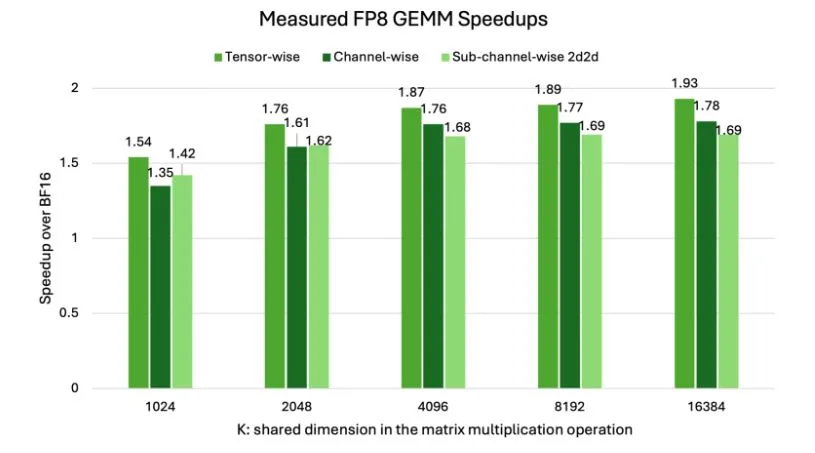
Figure 1 shows measured FP8 higher-precision matrix multiplications (GEMM) throughput speedup over BF16 for various scaling approaches on NVIDIA H100. Hardware-native scaling (channel-wise, subchannel-wise, tensor-wise) achieves up to 2x acceleration, underscoring why FP8 is so effective at the hardware level.
While FP8 offers significant speedups over BF16, the choice of scaling granularity; that is, how finely scaling factors are applied within a tensor introduces nuanced trade-offs in actual performance, particularly for GEMM operations. Finer granularity, while beneficial for numerical stability and accuracy by better accommodating intra-tensor variability, can introduce additional overhead that impacts raw throughput.
Figure 1. Higher-precision matrix multiplications (GEMM) speedups over BF16
A clear hierarchy in performance is observed when varying scaling granularities for GEMM operations. Tensor-wise scalinggenerally demonstrates the highest speedup. With only a single scaling factor per entire tensor involved in the GEMM, the overhead associated with scale management is minimized.
Channel-wise scalingrepresents an intermediate level of granularity, typically applying a scaling factor per channel or a row/column. As seen in the figure, its speedup falls between tensor-wise and 2D block-wise methods.
Sub-channel-wise 2D2D Scaling (for example, with 1×128 for activations and 128×128 blocks for weights)method, representing a finer granularity, generally exhibits slightly lower speedups compared to tensor-wise scaling. The management of multiple scaling factors for the many smaller blocks within a tensor introduces a computational cost that, while crucial for accuracy, can reduce peak raw throughput. This holds true for other configurable block dimensions like 1D1D or 1D2D, where finer block divisions mean more scales to process per GEMM.
Crucially, the x-axis in Figure 1 highlights the impact of GEMM size. As K increases (meaning larger GEMM operations), the overall speedup of FP8 over BF16 generally improves across all scaling methods. This is because for larger GEMMs, the computational savings from using 8-bit precision become more dominant, outweighing the relative overhead of managing scaling factors. In essence, larger GEMMs allow the inherent benefits of FP8 compute to shine through more effectively, even with the added complexity of finer-grained scaling.
While hardware-native solutions like MXFP8 are designed to mitigate the overhead of block scaling through dedicated Tensor Core acceleration, for general FP8 block scaling implementations, the trade-off between granularity (for accuracy) and raw performance remains a key consideration.
Beyond raw speedup, a critical aspect of low-precision training is convergence—how well the model learns and reduces its loss, and ultimately, how it performs on specific downstream tasks. While training loss provides valuable insight into the learning process, it’s important to remember that it’s not the sole metric for FP8 efficacy; robust FP8 downstream evaluation metrics are the ultimate arbiters of a model’s quality.
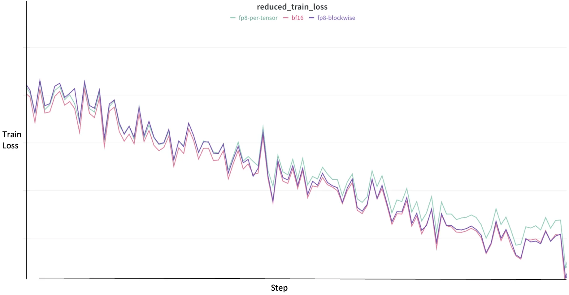
Figure 2. Training loss curves for FP8 techniques and BF16 on Llama 3.1
When adopting FP8, the expectation is that the training loss trajectory should closely mirror that of a higher-precision baseline, such as BF16, to ensure that the model is learning effectively without significant degradation. As shown in Figure 2, the training loss trajectories for different scaling strategies relative to BF16. The pink line represents the BF16 baseline. Notably, the dark purple line, representing FP8-blockwise scaling, consistently follows a trajectory very similar to BF16. This close alignment indicates that with finer granularity, block-wise scaling can preserve numerical fidelity more effectively, leading to a convergence behavior that closely matches the higher-precision BF16 training.
Conversely, the light green line, representing FP8-per-tensor scaling, occasionally shows slight deviations or higher fluctuations in loss. This subtle difference in convergence trajectory highlights the trade-off inherent in granularity: while coarser-grained per-tensor scaling might offer higher raw GEMM throughput as discussed previously, finer-grained block-wise scaling tends to yield less accuracy loss and a more stable learning path that closely mirrors BF16.
This illustrates the crucial balance between speedup and numerical stability in FP8 training. More granular scaling methods, by better accommodating the diverse dynamic ranges within tensors, can lead to convergence trajectories that more faithfully track higher-precision baselines, though this might come with a corresponding difference in speed compared to less granular approaches. The optimal choice often involves weighing the demands of downstream evaluation against available computational resources and desired training speed.
Experimental setup
All experiments in this post were conducted using NVIDIA NeMo Framework 25.04, the latest release of the NeMo framework at the time of writing. NeMo Framework 25.04 provides robust, production-grade support for FP8 training through the NVIDIA Transformer Engine (TE), and includes out-of-the-box recipes for dense architectures.
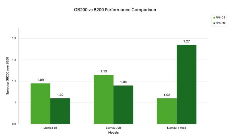
We evaluated two leading FP8 approaches: the current scaling recipe on H100 GPUs and the MXFP8 recipe on the newer NVIDIA DGX B200 architecture. For both, we tested a range of state-of-the-art models, including Llama 3 8B, Llama 3 70B, Llama 3.1 405B, Nemotron 15B, and Nemotron 340B. Each setup was compared directly against a BF16 baseline to measure the practical speedup delivered by FP8 in real-world training scenarios.
Current scaling recipe
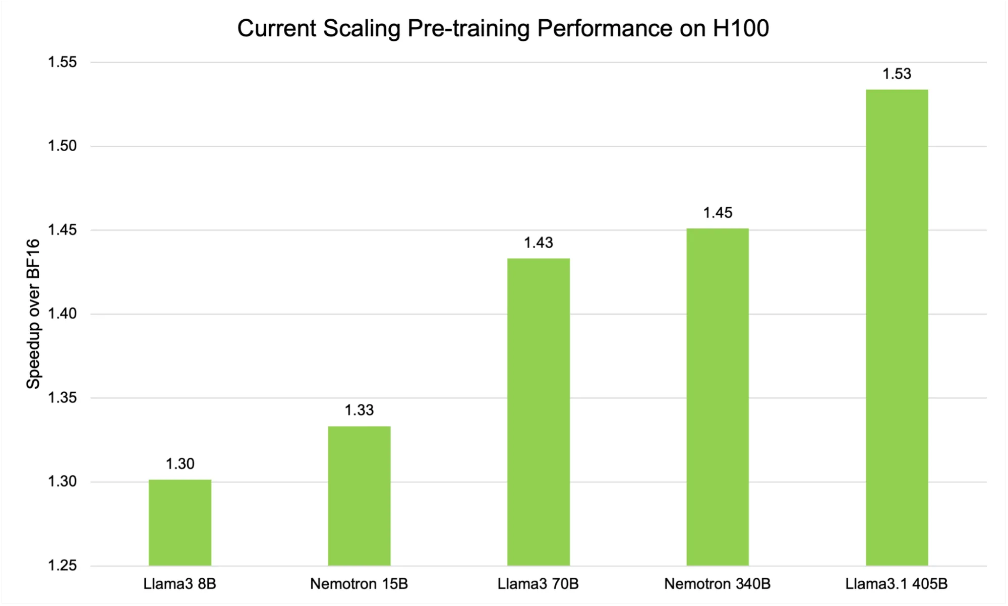
As illustrated in Figure 3, the current scaling FP8 recipe on H100 GPUs demonstrates a pronounced, model-size-dependent speedup when compared to the BF16 baseline. For smaller models such as Llama3 8B, the speedup is approximately 1.30x.
This advantage becomes even more significant with larger architectures. For example, the Llama 3 70B model achieves a speedup of 1.43x, and the largest model in our benchmark suite, Llama 3.1 405B, reaches an impressive 1.53x acceleration.
Figure 3. Model-size-dependent speedup with the current scaling FP8 recipe on H100 GPUs
This upward trend is not just a statistical curiosity—it underscores a fundamental advantage of FP8 training for large-scale language models. As model size and computational complexity increase, the efficiency gains from reduced-precision arithmetic become more pronounced.
The reason is twofold: First, larger models naturally involve more matrix multiplications and data movement, both of which benefit substantially from the reduced memory footprint and higher throughput of FP8 on modern hardware. Second, the overheads associated with scaling and dynamic range adjustments become relatively less significant as the total computation grows, allowing the raw performance benefits of FP8 to dominate.
MXFP8 recipe
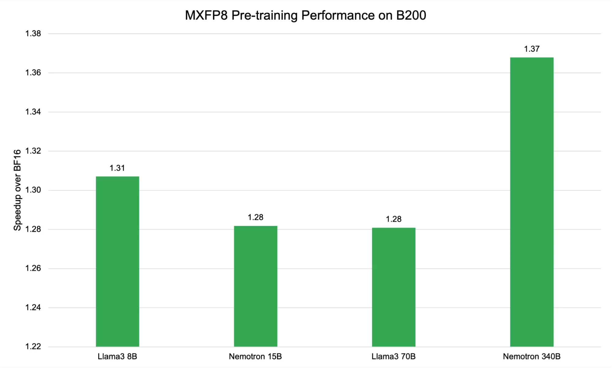
Figure 4 shows the performance of the MXFP8 recipe on DGX B200 GPUs, revealing a consistent speedup over BF16 across different model sizes, with observed gains ranging from 1.28x to 1.37x. While these absolute speedup values are slightly lower than those achieved by the current scaling recipe, they are notable for their stability and reliability across a diverse set of models.
Figure 4. Performance of the MXFP8 recipe on NVIDIA DGX B200 GPUs across model sizes
The relative flatness in speedup from 8B to 70B parameters—contrasted with the higher jump at 340B—reflects how block-based scaling interacts with model and hardware characteristics. MXFP8 assigns a shared scaling factor to each 32-element block, which can introduce additional memory access overhead for mid-sized models. However, as model size increases and computation becomes the dominant bottleneck (as seen with Nemotron 340B), the efficiency benefits of block-wise FP8 become more pronounced, leading to the observed peak speedup.
These results highlight the architectural strengths of the Blackwell (B200) platform, whose Tensor Cores and memory hierarchy are optimized for microscaling formats like MXFP8. This enables high throughput and stable convergence, even as models scale into the hundreds of billions of parameters. The block-level scaling approach of MXFP8 effectively balances dynamic range and computational efficiency, delivering reliable acceleration while mitigating risks of numerical instability.
This consistency reflects the architectural advancements of NVIDIA Blackwell architecture, which was purpose-built to maximize efficiency for lower-precision formats like FP8 and, specifically, for block-based scaling approaches such as MXFP8. The B200 Tensor Cores and advanced memory hierarchy are optimized for these microscaling formats, enabling high throughput and efficient memory utilization even as model sizes continue to increase. With MXFP8, each block of 32 values shares a scaling factor, striking a balance between dynamic range and computational efficiency. This approach allows for robust acceleration while minimizing the risk of numerical instability—a key consideration when pushing models to ever-larger scales.
How does NVIDIA GB200 Grace Blackwell Superchip compare to NVIDIA Blackwell architecture?
The comparison between GB200 and B200 highlights how architectural integration and system design can translate into tangible performance gains for large-scale AI workloads. Both are built on NVIDIA Blackwell architecture, but the GB200 superchip combines two B200 GPUs with a Grace CPU, interconnected through NVIDIA NVLink, resulting in a unified memory domain and exceptionally high memory bandwidth.
Figure 5. Speedup of GB200 over B200 for different model sizes and FP8 recipes. Note that the numbers shown here are computed with NeMo FW 25.04 and may change as further validation is performed
Get started with practical FP8 training
A clear pattern emerges from these benchmarks: for dense models, the bigger the model, the bigger the speedup with FP8. This is because as model size increases, the number of matrix multiplications (GEMMs) grows rapidly, and these operations benefit most from the reduced precision and higher throughput of FP8. In large dense models, FP8 enables dramatic efficiency gains, making it possible to train and fine-tune ever-larger language models with less time and compute.
These empirical results reinforce the specific strengths and tradeoffs of each FP8 scaling recipe detailed in this post and demonstrate that both per-tensor and MXFP8 approaches deliver significant speedup and convergence benefits over BF16.
Ready to try these techniques yourself? Explore the FP8 recipes to get started with practical FP8 training configurations and code.
Building a robust visual inspection pipeline for defect detection and quality control is not easy. Manufacturers and developers often face challenges such as customizing general-purpose vision AI models for specialized domains, optimizing the model size on compute‑constrained edge devices, and deploying in real time for maximum inference throughput.
NVIDIA Metropolis is a development platform for vision AI agents and applications that helps to solve these challenges. Metropolis provides the models and tools to build visual inspection workflows spanning multiple stages, including:
Customizing vision foundation models through fine-tuning
Optimizing the models for real‑time inference
Deploying the models into production pipelines
NVIDIA Metropolis provides a unified framework and includes NVIDIA TAO 6 for training and optimizing vision AI foundation models, and NVIDIA DeepStream 8, an end-to-end streaming analytics toolkit. NVIDIA TAO 6 and NVIDIA DeepStream 8 are now available for download. Learn more about the latest feature updates in the NVIDIA TAO documentation and NVIDIA DeepStream documentation.
This post walks you through how to build an end-to-end real-time visual inspection pipeline using NVIDIA TAO and NVIDIA DeepStream. The steps include:
Performing self-supervised fine-tuning with TAO to leverage domain-specific unlabeled data.
Optimizing foundation models using TAO knowledge distillation for better throughput and efficiency.
Deploying using DeepStream Inference Builder, a low‑code tool that turns model ideas into production-ready , standalone applications or deployable microservices.
How to scale custom model development with vision foundation models using NVIDIA TAO
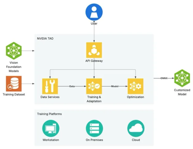
NVIDIA TAO supports the end-to-end workflow for training, adapting, and optimizing large vision foundation models for domain specific use cases. It’s a framework for customizing vision foundation models to achieve high accuracy and performance with fine-tuning microservices.
Figure 1. Use NVIDIA TAO to create highly accurate, customized, and enterprise-ready AI models to power your vision AI applications
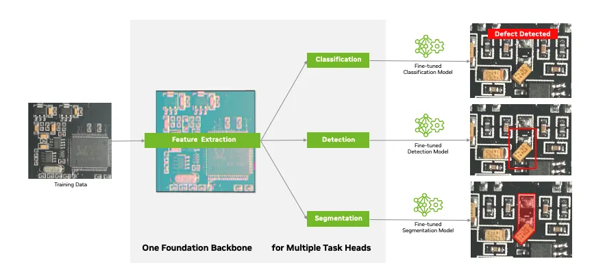
Vision foundation models (VFMs) are large-scale neural networks trained on massively diverse datasets to capture generalized and powerful visual feature representations. This generalization makes them a flexible model backbone for a wide variety of AI perception tasks such as image classification, object detection, and semantic segmentation.
TAO provides a collection of these powerful foundation backbones and task heads to fine-tune models for your key workloads like industrial visual inspection. The two key foundation backbones in TAO 6 are C-RADIOv2 (highest out-of-the-box accuracy) and NV-DINOv2. TAO also supports third-party models, provided their vision backbone and task head architectures are compatible with TAO.
Figure 2. Scale custom vision model development with NVIDIA TAO fine-tuning framework, foundation model backbones, and task heads
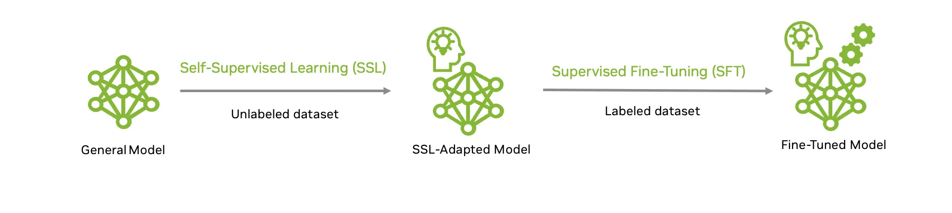
To boost model accuracy, TAO supports multiple model customization techniques such as supervised fine-tuning (SFT) and self-supervised learning (SSL). SFT requires collecting annotated datasets that are curated for the specific computer vision downstream tasks. Collecting high-quality labeled data is a complex, manual process that is time-consuming and expensive.
Second, NVIDIA TAO 6 empowers you to leverage self-supervised learning to tap into the vast potential of unlabeled images to accelerate the model customization process where labeled data is scarce or expensive to acquire.
This approach, also called domain adaption, enables you to build a robust foundation model backbone such as NV-DINOv2 with unlabeled data. This can then be combined with a task head and fine-tuned for various downstream inspection tasks with a smaller annotated dataset.
In practical scenarios, this workflow means a model can learn the nuanced characteristics of defects from plentiful unlabeled images, then sharpen its decision-making with targeted supervised fine-tuning, delivering state-of-the-art performance even on customized, real-world datasets.
Figure 3. End-to-end workflow to adapt a foundation model for a specific downstream use case
Boosting PCB defect detection accuracy with foundation model fine-tuning
To provide an example, we applied the TAO foundation model adaptation workflow using large-scale unlabeled printed circuit board (PCB) images to fine-tune a vision foundation model for defect detection. Starting with NV-DINOv2, a general-purpose model trained on 700 million general images, we customized it with SSL for PCB applications with a dataset of ~700,000 unlabeled PCB images. This helped transition the model from broad generalization, to sharp domain-specific proficiency.
Once domain adaptation is complete, we leveraged an annotated PCB dataset, using linear probing to refine the task-specific head for accuracy, and full fine-tuning to further adjust both backbone and a classification head. This first dataset consisted of around 600 training and 400 testing samples, categorizing images as OK or Defect (including patterns such as missing, shifts, upside-down, poor soldering, and foreign objects).
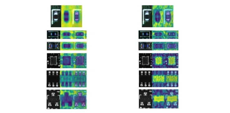
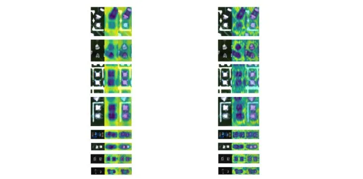
Feature maps show that the adapted NV-DINOv2 can sharply distinguish components and foreground-background (Figures 4 and 5) even before downstream fine-tuning. It excels in separating complex items like integrated circuit (IC) pins from the background—a task that’s not possible with a general model.
Figure 4. A comparison of feature maps for the OK class using the domain-adapted NV-DINOv2 (left) and the general NV-DINOv2 (right)Figure 5. A comparison of feature maps for the Defect class using the domain-adapted NV-DINOv2 (left) and the general NV-DINOv2 (right)
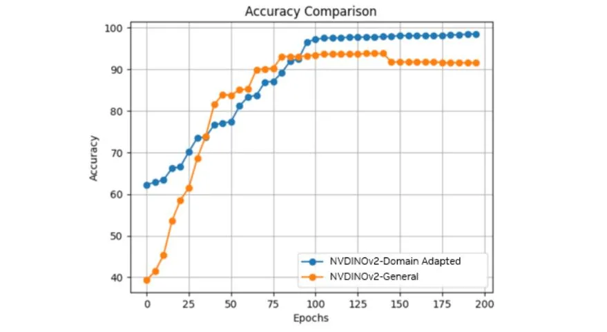
This results in substantial classification accuracy improvements of 4.7% from 93.8% to 98.5%.
Figure 6. Accuracy comparison between the domain-adapted and generic NV-DINOv2
The domain-adapted NV-DINOv2 also shows strong visual understanding and extracting relevant image features within the same domain. This indicates that similar or better accuracy can be achieved using less labeled data with downstream supervised fine-tuning.
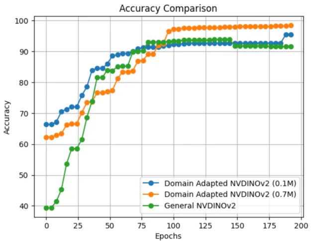
In certain scenarios, gathering such a substantial amount of data with 0.7 million unlabeled images could still be challenging. However, you could still benefit from NV-DINOv2 domain adaptation even with a smaller dataset.
Figure 7 shows the results of running an experiment adapting NV-DINOv2 with just 100K images, which also outperforms the general NV-DINOv2 model.
Figure 7. Accuracy comparison between different NV-DINOv2 models for classification
This example illustrates how leveraging self-supervised learning on unlabeled domain data using NVIDIA TAO with NV-DINOv2 can yield robust, accurate PCB defect inspection while reducing reliance on large amounts of labeled samples.
How to optimize vision foundation models for better throughput
Optimization is an important step in deploying deep learning models. Many generative AI and vision foundation models could have hundred million parameters which make them compute hungry and too big for most edge devices that are used in real-time applications such as industrial visual inspection or real-time traffic monitoring systems.
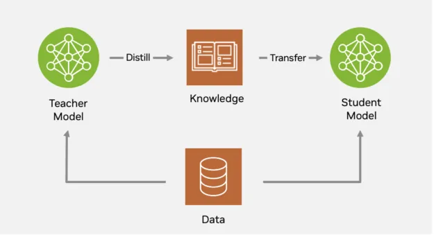
NVIDIA TAO leverages knowledge from these larger foundation models and optimizes them into smaller model sizes using a technique called knowledge distillation. Knowledge distillation compresses large, highly-accurate teacher models into smaller, faster student models, often without losing accuracy. This process works by having the student mimic not just the final predictions, but also the internal feature representations and decision boundaries of the teacher, making deployment practical on resource-constrained hardware and enabling scalable model optimization.
NVIDIA TAO takes knowledge distillation further with its robust support for different forms, including backbone, logit, and spatial/feature distillation. A standout feature in TAO is its single-stage distillation approach, designed specifically for object detection. With this streamlined process, a student model—often much smaller and faster—learns both backbone representations and task-specific predictions directly from the teacher in one unified training phase. This enables dramatic reductions in inference latency and model size, without sacrificing accuracy.
Applying single-stage distillation for a real-time PCB defect detection model
The effectiveness of distillation using TAO was evaluated on a PCB defect detection dataset comprising 9,602 training images and 1,066 test images, covering six challenging defect classes: missing hole, mouse bite, open circuit, short, spur, and spurious copper. Two distinct teacher model candidates were used to evaluate the distiller. The experiments were performed with backbones that were initialized from the ImageNet-1K pretrained weights, and results were measured based on the standard COCO mean Average Precision (mAP) for object detection.
Figure 8. Use NVIDIA TAO to distill knowledge from a larger teacher model into a smaller student model
In our first set of experiments, we ran the same distillation experiments using the ResNet series of backbones in the teacher-student combination, where the accuracy of student models not only matches but can even exceed their teacher model’s accuracy.
The baseline experiments are run as train actions associated with the RT-DETR model in TAO. The following snippet shows a minimum viable experiment spec file that you can use to run a training experiment.
tao model rtdetr train -e /path/to/experiment/spec.yaml results_dir=/path/to/results/dir model.backbone=backbone_name model.pretrained_backbone_path=/path/to/the/pretrained/model.pth
You can change the backbone by overriding the model.backbone parameter to the name of the backbone and model.pretrained_backbone_path to the path to the pretrained checkpoint file for the backbone.
A distillation experiment is run as a distill action associated with the RT-DETR model in TAO. To configure the distill experiment, you can add the following config element to the original train experiment spec file.
Run distillation using the following sample command:
tao model rtdetr distill -e /path/to/experiment/spec/yaml results_dir=/path/to/results/dir model.backbone=backbone_namemodel.pretrained_backbone_path=/path/to/pretrained/backbone/checkpoint.pth distill.teacher.backbone=teacher_backbone_name distill.pretrained_teacher_model_path=/path/to/the/teacher/model.pth
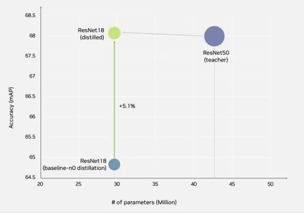
Figure 9. Distilling a ResNet50 model into a lighter ResNet18 model yields a 5% accuracy gain
While deploying a model on edge, both inference acceleration and memory limit could be of significant consideration. TAO enables distilling detection features not just within the same family of backbones, but also across backbone families.
Figure 10. Distilling a ConvNeXt model into a lighter ResNet34-based model yields a 3% accuracy gain
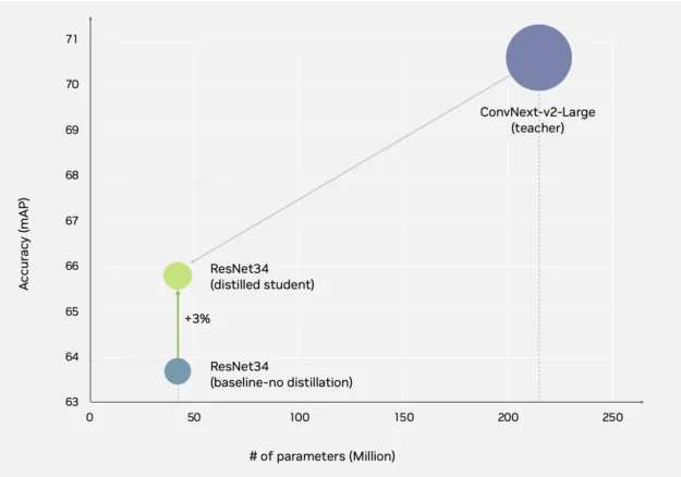
In this example, we used a ConvNeXt based RT-DETR model as the teacher and distilled it to a lighter ResNet34-based model. Through single-stage distillation, TAO improved accuracy by 3%, reducing the model size by 81% for higher throughput, low-latency inference.
How to package and deploy models with DeepStream 8 Inference Builder
Now with a trained and distilled RT-DETR model from TAO, the next step is to deploy it as an inference microservice. The new NVIDIA DeepStream 8 Inference Builder is a low‑code tool that turns model ideas into standalone applications or deployable microservices.
To use the Inference Builder, provide a YAML configuration, a Dockerfile and an optional OpenAPI definition. The Inference Builder then generates Python code that connects the data loading, GPU‑accelerated preprocessing, inference, and post‑processing stages, and can expose REST endpoints for microservice deployments.
It is designed to automate the generation of inference service code, API layers, and deployment artifacts from a user-provided model and configuration files. This eliminates the need for manual development of boilerplate code pertaining to servers, request handling, and data flow, as a simple configuration suffices for Inference Builder to manage these complexities.
Video 1. Learn how to deploy AI models using the NVIDIA DeepStream Inference Builder
Step 1: Define the configuration
Create a config.yaml file to delineate your model and inference pipeline
(Optional) Incorporate an openapi.yaml file if explicit API schema definition is desired
Step 2: Execute the DeepStream Inference Builder
Submit the configuration to Inference Builder
This utility leverages inference templates, server templates, and utilities (codec, for example) to autonomously generate project code
The output constitutes a comprehensive package, encompassing inference logic, server code, and auxiliary utilities
Output infer.tgz, a packaged inference service
Step 3: Examine the generated code
The package expands into a meticulously organized project, featuring:
Configuration: config/
Server logic: server/
Inference library: lib/
Utilities: asset manager, codec, responders, and so on
Step 4: Construct a Docker image
Use the reference Dockerfile to containerize the service
Execute docker build -t my-infer-service
Step 5: Deploy with Docker Compose
Initiate the service using Docker Compose: docker-compose up
The service will subsequently load your models within the container
Step 6: Serve to users
Your inference microservice is now operational
End users or applications can dispatch requests to the exposed API endpoints and receive predictions directly from your model
To learn more about the NVIDIA DeepStream Inference Builder, visit NVIDIA-AI-IOT/deepstream_tools on GitHub.
Additional applications for real-time visual inspection
In addition to identifying PCB defects you can also apply TAO and DeepStream to spot anomalies in industries such as automotive and logistics. To read about a specific use case, see Slash Manufacturing AI Deployment Time with Synthetic Data and NVIDIA TAO.
Get started building a real-time visual inspection pipeline
With NVIDIA DeepStream and NVIDIA TAO, developers are pushing the boundaries of what’s possible in vision AI—from rapid prototyping to large-scale deployment.
DeepStream 8.0 equips developers with powerful tools like the Inference Builder to streamline pipeline creation and improve tracking accuracy across complex environments. TAO 6 unlocks the potential of foundation models through domain adaptation, self-supervised fine-tuning, and knowledge distillation.
This translates into faster iteration cycles, better use of unlabeled data, and production-ready inference services.
Ready to get started?
Download NVIDIA TAO 6 and explore the latest features. Ask questions and join the conversation in the NVIDIA TAO Developer Forum.
Download NVIDIA DeepStream 8 and explore the latest features. Ask questions and join the conversation in the NVIDIA DeepStream Developer Forum.
Tantangan yang berulang dalam desain molekuler, baik untuk aplikasi farmasi, kimia, atau material, adalah membuat molekul yang dapat disintesis. Penilaian Sintesizabilitas Seringkali membutuhkan pemetaan jalur sintesis untuk suatu molekul: urutan reaksi kimia yang diperlukan untuk mengubah molekul prekursor menjadi molekul produk target. Posting ini memperkenalkan Rasyn, model generatif dari NVIDIA yang dirancang untuk memprediksi jalur sintesis molekuler yang juga membahas keterbatasan dalam pendekatan saat ini.
Mengapa Penalaran Rantai Pikiran Masalah untuk AI dalam Kimia
Model Bahasa Besar (LLM) telah menjadi bagian integral dari kehidupan sehari-hari, memberi daya pada aplikasi dari asisten virtual ke pemecahan masalah yang kompleks. LLM modern memecahkan masalah kompleks dengan menghasilkan rantai pemikiran (COT), yang merupakan serangkaian langkah penalaran perantara yang mengarah pada jawaban akhir. Menggabungkan metode pencarian COT dan waktu tes, seperti menghasilkan beberapa jalur COT, sangat penting untuk peningkatan akurasi LLM terbaru.
Kimia menghadapi tantangan yang sama dalam prediksi jalur sintesis molekuler, di mana jalur berisi serangkaian langkah sintesis menengah. Prediksi jalur adalah langkah penting dalam pengembangan obat, bahan kimia, dan bahan karena molekul, betapapun menjanjikannya, hanya berharga jika dapat disintesis. Reasyn adalah kerangka generatif baru yang secara efisien memprediksi jalur sintesis molekuler. Ini menggunakan notasi rantai reaksi (COR) yang unik, yang terinspirasi oleh pendekatan COT di LLMS, dikombinasikan dengan algoritma pencarian waktu tes.
Jalur sintetis mengikuti struktur pohon bottom-up: molekul sederhana, atau blok bangunan (BB), digabungkan melalui reaksi kimia (RXN) untuk menghasilkan produk menengah (INT), yang pada gilirannya mengalami reaksi lebih lanjut untuk membentuk molekul yang semakin kompleks (Gambar 1). Proses ini multi-langkah, dengan setiap reaksi diterapkan pada reaktan yang mungkin merupakan blok bangunan atau perantara. Dalam praktiknya, ahli kimia menyimpulkan jalur seperti itu langkah demi langkah, alasan melalui setiap transformasi untuk mencapai molekul target akhir.
Gambar 1. Notasi Cor melihat jalur sintetis sebagai jalur penalaran ranjang
Rasyn menangkap penalaran langkah demi langkah ini melalui notasi cor-nya, terinspirasi oleh pendekatan COT di LLMS. Di COR, seluruh jalur sintetis direpresentasikan sebagai urutan linier di mana setiap langkah secara eksplisit mencakup reaktan, aturan reaksi, dan produk yang dihasilkan. Reaktan dan produk dikodekan sebagai senyum (string, dibungkus dengan token khusus yang menandai batas mereka), sementara setiap reaksi dilambangkan dengan token kelas reaksi tunggal. Representasi ini tidak hanya mencerminkan bagaimana ahli kimia berpikir tentang sintesis tetapi juga memungkinkan model untuk menerima pengawasan menengah pada setiap langkah untuk belajar lebih kaya aturan reaksi kimia dan pembuatan jalur multi-langkah yang lebih andal.
Gambar 2. Kerangka kerja keseluruhan dari RECYN
Membangun di atas notasi COR dan desain berurutan, Reasyn beroperasi sebagai model generatif autoregresif (Gambar 2) yang memperlakukan jalur sintetis sebagai rantai penalaran – masing -masing langkah yang sesuai dengan reaksi kimia tunggal. Sama seperti penalaran COT di LLMS menghasilkan langkah -langkah perantara sebelum jawaban akhir, Reasyn secara bertahap membangun jalur mulai dari blok bangunan sederhana ke molekul target. Ini memungkinkannya untuk merekonstruksi jalur untuk molekul yang dapat disintesis dan ke proyek Molekul yang tidak dapat disinkronkan ke dalam ruang kimia yang dapat disintesis, memproduksi analog yang dapat disintesiskan yang dapat dibuat dalam praktiknya.
Setelah model memprediksi reaktan dan aturan reaksi pada setiap langkah, produk menengah dapat dengan mudah diperoleh dengan menggunakan pelaksana reaksi seperti RDKI. Informasi menengah ini tidak hanya memberikan sinyal pelatihan yang lebih kaya untuk model untuk mempelajari aturan kimia, tetapi juga memandu proses pembuatan jalur sintetis.
Melihat generasi jalur sintetis sebagai penalaran LLM juga memungkinkan kami untuk mengadopsi teknik penalaran LLM tambahan seperti penguatan pembelajaran (RL) finetuning dan pencarian waktu tes. Rasyn mengeksplorasi dua teknik ini untuk generasi jalur sintetis.
Bagaimana RL Finetuning Berbasis Hasil Meningkatkan Eksplorasi
Mungkin ada beberapa jalur yang mengarah ke molekul produk yang sama. Reasyn mendapat manfaat dari pengambilan sampel berbagai jalur sintetis dan mendapatkan umpan balik melalui GRPO). Hadiah berbasis hasil untuk jalur diatur ke kesamaan molekuler antara molekul produk akhir dan molekul input. Karena hadiah hanya diterapkan pada hasilnya, alih -alih langkah -langkah penalaran, model ini diberkahi dengan kemampuan untuk mengeksplorasi berbagai jalur sintetis.
Gambar 3. Pembelajaran Penguatan (RL) Finetuning dari RECYN Menggunakan GRPO
Pencarian yang diarahkan pada tujuan: jalur panduan
Selama generasi, Reasyn menggunakan pencarian balok, yang mempertahankan kumpulan urutan yang dihasilkan dan memperluasnya blok demi blok (BB atau RXN). Pencarian memungkinkan RECYN untuk menghasilkan beragam jalur untuk molekul input tunggal, dan memandu generasi dalam arah yang disukai dengan mencetak urutan melalui fungsi hadiah. Dalam perencanaan retrosintesis, fungsi hadiah dapat menjadi kesamaan dengan molekul input. Dalam tugas optimasi yang diarahkan pada tujuan, fungsi hadiah dapat menjadi properti kimia yang diinginkan.
Gambar 4. Pencarian waktu tes yang diarahkan pada tujuan dari Rasyn
Menghasilkan jalur sintetis dengan reasyn
Proyeksi Sintesizable Reasyn sangat fleksibel: memungkinkan perencanaan retrosintesis, menyarankan analog untuk molekul yang tidak dapat disinkronkan, mendukung optimasi molekuler yang diarahkan pada tujuan, dan memfasilitasi ekspansi hit yang dapat disintesis. Di bawah ini, kami memeriksa kinerjanya pada tugas -tugas ini.
Perencanaan retrosintesis
Tabel 1. Tingkat keberhasilan perencanaan retrosintesis (%)
Bahkan dengan ruang yang dapat disintesiskan secara luas, metode pembuatan molekul yang dapat disintesis sebelumnya telah berjuang untuk menutupi ruang ini secara luas. Rasyn menunjukkan tingkat keberhasilan yang tinggi dalam menghasilkan jalur sintetis yang diberikan molekul yang dapat disintesis, menunjukkan eksplorabilitasnya yang kuat dalam ruang kimia yang dapat disintesis.
Optimalisasi molekul yang diarahkan sasaran yang dapat disintalkan
Tabel 2. Rata -rata skor optimasi yang dapat disintesis dari tugas optimasi molekuler 15 pmo
Reasyn dapat memproyeksikan molekul yang dihasilkan oleh metode optimasi molekuler di luar rak untuk melakukan optimasi yang diarahkan pada tujuan yang dapat disintesi. Dikombinasikan dengan grafik GA, grafik GA-Reasyn menunjukkan kinerja optimasi yang lebih tinggi daripada metode berbasis sintesis sebelumnya.
Ekspansi hit yang dapat disintesis: Menjelajahi lingkungan molekul
Skema pencarian memungkinkan RECYN untuk menyarankan beberapa analog yang dapat disintesis untuk molekul target yang diberikan dengan memproyeksikannya secara berbeda. RECYN mengeksplorasi lingkungan molekul yang diberikan dalam ruang yang dapat disintesis, dan dapat diterapkan untuk menghitung ekspansi untuk menemukan analog yang dapat disintesis dari molekul hit (Gambar 5).
Gambar 5. Ekspansi hit yang dapat disintesis dengan Reasyn
Sebagian besar model generatif menciptakan molekul yang tidak dapat disintesional dalam praktiknya. Rasyn membangun kemajuan penalaran baru -baru ini di LLMS, melengkapi para ilmuwan dengan alat generatif yang efektif untuk memproyeksikan molekul kecil ke dalam ruang kimia yang dapat disintesis. Dengan peningkatan kemampuan penalaran, keanekaragaman, dan keserbagunaan, Reasyn menunjukkan janji sebagai sarana untuk menavigasi ruang kimia yang dapat disintesis secara kombinatorial dalam penemuan obat dunia nyata.
Cari tahu lebih lanjut tentang Reasyn dengan membaca makalah kami tentang ARXIV dan kode tersedia di GitHub.
Unlike traditional LLM-based systems that are limited by their training data, retrieval-augmented generation (RAG) improves text generation by incorporating relevant external information. Agentic RAG goes a step further by leveraging autonomous systems integrated with LLMs and retrieval mechanisms. This allows these systems to make decisions, adapt to changing requirements, and perform complex reasoning tasks dynamically.
In this guide to the self-paced workshop for building a RAG agent, you’ll gain:
Understanding of the core principles of agentic RAG, including NVIDIA Nemotron, an open model family with open data and weights.
Knowledge of how to build agentic RAG systems using LangGraph.
A turnkey, portable development environment.
Your own customized agentic RAG system, ready to share as an NVIDIA Launchable.
Video walkthrough
Video 1. Build a RAG Agent with NVIDIA Nemotron
Opening the workshop
Launch the workshop as an NVIDIA Launchable:
Figure 1. Click on the ‘Deploy Now’ button to deploy the NVIDIA DevX Workshop in the cloud
With your Jupyter Lab environment running, locate the NVIDIA DevX Learning Path section of the Jupyterlab Launcher. Select the Agentic RAG tile to open up the lab instructions and get started.
Figure 2. Click on the “Agentic RAG” tile in NVIDIA DevX Learning Path to open lab instructions.
Setting up secrets
In order to follow along with this workshop, you’ll need to gather and configure a few project secrets.
NGC API Key: This enables access to NVIDIA software, models, containers, and more
(optional) LangSmith API Key: This connects the workshop to LangChain’s platform for tracing and debugging your AI Agent
You can utilize the Secrets Manager tile under NVIDIA DevX Learning Path of the Jupyterlab Launcher to configure these secrets for your workshop development environment. Verify in the logs tab that the secrets have been added successfully.
Figure 3. Use the “Secrets Manager” tile under the NVIDIA DevX Learning Path section to configure project secrets (API keys).
Introduction to RAG architecture
Once your workshop environment has been set up, the next step is understanding the architecture of the agentic RAG system you’ll build.
RAG enhances the capabilities of LLMs by incorporating relevant external information during output text generation. Traditional language models generate responses based solely on the knowledge captured in their training data, which can be a limiting factor, especially when dealing with rapidly changing information, highly specialized knowledge domains, or enterprise confidential data. RAG, on the other hand, is a powerful tool for generating responses based on relevant unstructured data retrieved from an external knowledge base.
Figure 4. Traditionally, RAG utilizes a user prompt to retrieve contextually-relevant documents, providing them as context to the LLM for a more informed response.
The typical flow for a RAG system is:
Prompt: A user generates a natural language query.
Embedding Model: The prompt is converted into vectors
Vector Database Search: After a user’s prompt is embedded into a vector, the system searches a vector database filled with semantically indexed document chunks, enabling fast retrieval of contextually relevant data chunks.”
Reranking Model: The retrieved data chunks are reranked to prioritize the most relevant data.
LLM: The LLM generates responses informed by the retrieved data.
This approach ensures that the language model can access up-to-date and specific information beyond its training data, making it more versatile and effective.
Understanding ReAct agent architecture
Unlike traditional LLM-based applications, agents can dynamically choose tools, incorporate complex reasoning, and adapt their analysis approach based on the situation at hand.
Figure 5. A ReAct agent can iteratively reason and call out to user-defined tools to generate a higher quality RAG-based response.
ReAct Agents are a simple agentic architecture that use “reasoning and acting” via tool calling supported LLMs. If the LLM requests any tool calls after taking in the prompt, those tools will be run, added to the chat history, and sent back to the model to be invoked again.
RAG works well, but it’s limited because the LLM can’t determine how data is retrieved, control for data quality, or choose between data sources. Agentic RAG takes the concept of RAG a step further by combining the strengths of LLMs such as language comprehension, contextual reasoning, and flexible generation, with dynamic tool usage, and advanced retrieval mechanisms such as semantic search, hybrid retrieval, reranking, and data source selection. Making a ReAct Agent for RAG just requires giving it the Retrieval Chain as a tool so the agent can decide when and how to search for information.
Figure 6. The full agentic RAG pipeline will involve adding the ReAct agent to the Retrieval Chain where the contextual documents are stored.
Agentic RAG employs a ReAct agent architecture in which the reasoning LLM systematically decides whether to retrieve information via tool calling or respond directly, activating the retrieval pipeline only when additional context is needed to better address the user’s request.
Learn and implement the code
Now that we understand the concepts, let’s dive into the technical implementation. We’ll start with the foundational components before building up to the complete agentic RAG system:
Models
Tools
Data Ingestion
Text Splitting
Vector Database Ingestion
Document Retriever and Reranker
Retriever Tool Creation
Agent Configuration
Foundations: the models
The workshop relies on NVIDIA NIM endpoints for the core model powering the agent. NVIDIA NIM provides high-performance inference capabilities, including:
Tool binding: Native support for function calling.
Structured output: Built-in support for Pydantic models.
Async operations: Full async/await support for concurrent processing.
To ensure the quality of the LLM-based application, it’s crucial that the agent receives clear instructions to clarify decision-making, remove ambiguity, and clarify how it should treat retrieved documents. One such example from code/rag_agent.py is provided as follows:
SYSTEM_PROMPT = (
    "You are an IT help desk support agent.\n"
    "- Use the 'company_llc_it_knowledge_base' tool for questions likely covered by the internal IT knowledge base.\n"
    "- Always write grounded answers. If unsure, say you don't know.\n"
    "- Cite sources inline using [KB] for knowledge base snippets.\n"
    "- If the knowledge base doesn't contain sufficient information, clearly state what information is missing.\n"
    "- Keep answers brief, to the point, and conversational."
)
This prompt shows a few key principles of reliable LLM prompting for RAG-based applications:
Role specification: Clear definition of the agent’s expertise and responsibilities.
Tool Utilization: Instruct the agent on which tools to use for specific tasks.
Grounding: Emphasize the importance of providing answers based on reliable sources and the importance of admitting to uncertainty.
Source Citation: Provide guidelines for citing sources to ensure transparency.
Communication Style: Specify the desired communication style.
In code/rag_agent.py we define the models necessary for the IT Help Desk agent to answer user queries by utilizing the Knowledge Base.
The LLM Model, Nemotron Nano 9b V2, is the primary reasoning model used for generating responses.
The NVIDIA NeMo Retriever Embedding Model, Llama 3.2 EmbedQA 1b V2, is used for converting documents into vector embedding representations for storage and retrieval.
The NeMo Retriever Reranking Model, Llama 3.2 RerankQA 1b V2, is used for reranking for the most relevant retrieved documents and data.
These models collectively enable the IT Help Desk agent to answer user queries accurately by leveraging a combination of language generation, document retrieval, and reranking capabilities.
Foundations: the tools
Our RAG agent will have access to the knowledge base provided at ./data/it-knowledge-base that contains markdown files documenting common IT-related procedures. The retriever tool enables the agent to search the internal IT knowledge base for documents relevant to the user’s query.
A vector database stores, indexes, and queries numerical representations of vectorized embeddings, allowing for fast similarity searches of unstructured data like text, images, and audio. For our purposes, we use an in-memory FAISS database, which is efficient for spinning up small databases. In terms of data ingestion to utilize the data in the knowledge base, we’ll focus on text ingestion. Additional features like multimodality should be considered for production use cases.
Foundations: data ingestion
The embedding model utilized is NeMo Retriever llama-3.2-nv-embedqa-1b-v2. This model creates embeddings for documents and queries that help in efficiently retrieving relevant documents from the knowledge base by comparing the semantic similarity between the query and the documents.
To ingest the documents, we’ll chunk the documents, embed those chunks into vectors, and then insert the vectors into the database. Before doing that, we need to load the data from our ./data/it-knowledge-base directory using the LangChain DirectoryLoader.
from langchain_community.document_loaders import DirectoryLoader, TextLoader
# Read the data
_LOGGER.info(f"Reading knowledge base data from {DATA_DIR}")
data_loader = DirectoryLoader(
    DATA_DIR,
    glob="**/*",
    loader_cls=TextLoader,
    show_progress=True,
)
docs = data_loader.load()
Foundations: text splitting
Document splitting is controlled by two things: chunk size and chunk overlap.
Chunk size defines the maximum length of each text chunk. This ensures that each chunk is of an optimized size for processing by language models and retrieval systems. A chunk size that is too large may contain information less relevant to specific queries, while one too small may miss important context.
Chunk overlap defines the number of tokens that overlap between consecutive chunks. The goal is to ensure continuity and preserve context across chunks, thereby maintaining coherence in the retrieved information.
To perform text splitting efficiently, we use the RecursiveCharacterTextSplitter. This tool recursively splits documents into smaller chunks based on character length, so each chunk adheres to the defined chunk size and overlap parameters. It’s particularly useful for processing large documents, improving the information retrieval’s overall accuracy.
To facilitate efficient retrieval of relevant information, we need to ingest our large corpus of documents into a vector database. Now that we have broken down our documents into manageable chunks, we utilize the embedding model to generate vector embeddings for each document chunk.
These embeddings are numerical representations of the semantic content of the chunks. High-quality embeddings enable efficient similarity searches, allowing the system to quickly identify and retrieve the most relevant chunks in response to a user’s query.
The next step is to store the generated embeddings in an in-memory FAISS database, which ensures fast indexing and querying capabilities for real-time information retrieval. In this example, we leverage the fact that LangChain’s FAISS `from_documents` method conveniently generates the embeddings for the document chunks and also stores them in the FAISS vector store in one function call.
from langchain_community.vectorstores import FAISS
from langchain_nvidia_ai_endpoints import NVIDIAEmbeddings,

embeddings = NVIDIAEmbeddings(model=RETRIEVER_EMBEDDING_MODEL, truncate="END")
vectordb = FAISS.from_documents(chunks, embeddings)
By following these steps and taking advantage of the power of the embedding model, we ensure that the IT Help Desk agent can efficiently retrieve and process relevant information from the knowledge base.
Foundations: document retriever and reranker
With our vector database populated, we can build a chain for content retrieval. This involves creating a seamless workflow that includes both the embedding step and the lookup step.
Figure 7. A basic retrieval chain consists of an embedding model and a database to store the converted vector embeddings.
In the embedding step, user queries are converted into embeddings using the same model that we previously used for document chunks. This ensures that both the queries and document chunks are represented in the same semantic space, enabling accurate similarity comparisons.
To initialize the retriever in this example, we’ll use semantic similarity and search for the top six returned results compared to our query.
The embeddings of the user’s queries are compared against the embeddings stored in the vector database during the lookup step. The system retrieves the most similar document chunks, which are then used to generate responses.
Figure 8. A more complex retrieval chain consists of attaching a Reranking model to reorganize retrieved context to put the most relevant chunks first.
For both the embedding and the reranking models, we’ll use NIM microservices from NVIDIA NeMo Retriever. LangChain allows us to easily create a basic retrieval chain from our Vector Database object that has both the embedding step and the lookup step.
For improving the relevance and order of retrieved documents, we can utilize the NVIDIA Rerank class, built on the NVIDIA NeMo Retriever Reranker model. The Reranker model evaluates and ranks the retrieved document chunks based on their relevance to the user’s query so that the most pertinent information is presented to the user first. In this example, we initialize the Reranker as follows:
from langchain_nvidia_ai_endpoints import NVIDIARerank
reranker = NVIDIARerank(model=RETRIEVER_RERANK_MODEL)
Foundations: Retriever tool creation
Taking the document retriever and the documenter reranker, we can now create the final document retriever as below:
The LangChain ContextualCompressionRetriever makes it easy to combine a retriever with additional processing steps, attaching the retrieval chain to the reranking model. Now we can create the retriever tool that enables our ReAct Agent.
In this example, we can initialize the retriever tool by using the LangChain tools package below, passing in our initialized retriever:
from langchain.tools.retriever import create_retriever_tool
RETRIEVER_TOOL = create_retriever_tool(
    retriever=RETRIEVER,
    name="company_llc_it_knowledge_base",
    description=(
        "Search the internal IT knowledge base for Company LLC IT related questions and policies."
    ),
)
Foundations: agent configuration
With our vector database and retriever chain in place, we’re ready to construct the agent graph. This agent graph acts as a kind of flowchart, mapping out the possible steps the model can take to accomplish its task. In traditional, step-by-step LLM applications, these are called “chains.” When the workflow involves more dynamic, non-linear decision-making, we refer to them as “graphs.” The agent can choose different paths based on the context and requirements of the task at hand, branching out into different decision nodes.
Given the prevalence of the ReAct agent architecture, LangGraph provides a function that’ll create ReAct Agent Graphs. In this example, we utilized as below:
By constructing an agent graph, we create a dynamic and flexible workflow that enables our IT Help Desk agent to handle complex decision-making processes. This approach ensures that the agent can efficiently retrieve and process information, provide accurate responses, and adapt to various scenarios.
Running your agent
Congratulations! You have successfully built your agent! Now, the next step is to try it out.
To get started with running your agent from your terminal, cd into the code directory that has the Python file containing your code for the agent. Once there, start your Agent API with the LangGraph CLI. Your agent will automatically reload as you make changes and save your code.
To chat with your agent, a simple Streamlit app has been included in the Simple Agents Client. You can also access the Streamlit Client from the Jupyter Launcher page. In the sidebar, ensure the rag_agent client is selected and try chatting!
Figure 9. Click on the “Simple Agents Client” tile in NVIDIA DevX Learning Path to open the Streamlit chat application.
As your agents become more sophisticated, managing their internal complexity can become difficult. Tracing helps visualize each step your agent takes, which makes it easier to debug and optimize your agent’s behavior. In the workshop, you can optionally configure the LANGSMITH_API_KEY and view traces on the LangSmith dashboard.
Migrate to local NIM microservices
This workshop utilizes the nvidia-nemotron-nano-9b-v2 LLM from the NVIDIA API Catalog. These APIs are useful for evaluating many models, quick experimentation, and getting started is free. However, for the unlimited performance and control needed in production, deploy models locally with NVIDIA NIM microservice containers.
In a typical development workflow, both your agent and NIM containers would run in the background, allowing you to multitask and iterate quickly. For this exercise, we can run the NIM in the foreground to easily monitor its output and ensure proper start up.
First, you need to log in to the NGC container registry as follows:
The next step is to create a location for NIM containers to save their downloaded model files.
docker volume create nim-cache
Now, we need to use a Docker run command to pull the NIM container image and model data files before hosting the model behind a local, OpenAI-compliant API.
With your langgraph server still running, go back to our Simple Agents Client and try prompting the agent again. If everything was successful, you should notice no change!
Congratulations! You have now migrated to using Local NIM microservices for your LangGraph Agent!
Conclusion and next steps
This workshop provides a comprehensive path from basic concepts to sophisticated agentic systems, emphasizing hands-on learning with production-grade tools and techniques.
By completing this workshop, developers gain practical experience with:
Fundamental concepts: Understanding the difference between standard and agentic RAG.
State management: Implementing complex state transitions and persistence.
Tool integration: Creating and managing agentic tool-calling capabilities.
Modern AI stack: Working with LangGraph, NVIDIA NIM, and associated tooling.
Learn More
For hands-on learning, tips, and tricks, join our Nemotron Labs livestream, “Build a RAG Agent with NVIDIA Nemotron” on Tuesday, September 23, 2025 at 9am PT.
Stay up to date on Agentic AI, Nemotron, and more by subscribing to NVIDIA news, joining the community, and following NVIDIA AI on LinkedIn, Instagram, X, and Facebook.
Explore the self-paced video tutorials and livestreams here.
Yang terbaru untuk devs dari made by google, pembaruan ke Gemini di Android Studio, ditambah androidify baru: episode musim panas kami dari The Android Show
Diposting oleh Matthew McCullough – VP manajemen produk, pengembang Android dalam ekosistem yang dinamis dan kompleks ini, komitmen kami adalah untuk …


 blog%20Assets_Hero%20banner.png”/>