03 Sep 2025
Jaringan Utara -Selatan: Kunci untuk beban kerja AI perusahaan yang lebih cepat
9 menit dibaca
Hardware Dan SoftWare Komputer
Mengenal prangkat-perangkat lunak serta keras dalam teknology dunai komputer
03 Sep 2025
Jaringan Utara -Selatan: Kunci untuk beban kerja AI perusahaan yang lebih cepat
9 menit dibaca
Mempercepat pengembangan dengan rilis bulanan untuk Android Studio – merilis 2x lebih sering dari sebelumnya
Diposting oleh Xavier Ducrohet – Tech Lead, Android Studio dan Adarsh Fernando – Group Product Manager, Android Studio tahun lalu, We Doubl …
Android
Plugin Android Gradle
Generating text with large language models (LLMs) often involves running into a fundamental bottleneck. GPUs offer massive compute, yet much of that power sits idle because autoregressive generation is inherently sequential: each token requires a full forward pass, reloading weights, and synchronizing memory at every step. This combination of memory access and step-by-step dependency raises latency, underutilizes hardware, and limits system efficiency.
Speculative decoding helps break through this wall. By predicting and verifying multiple tokens simultaneously, this technique shortens the path to results and makes AI inference faster and more responsive, significantly reducing latency while preserving output quality. This post explores how speculative decoding works, when to use it, and how to deploy the advanced EAGLE-3 technique on NVIDIA GPUs.
Speculative decoding is an inference optimization technique that pairs a target model with a lightweight draft mechanism that quickly proposes several next tokens. The target model verifies those proposals in a single forward pass, accepts the longest prefix that matches its own predictions, and continues from there. Compared with standard autoregressive decoding, which produces one token per pass, this technique lets the system generate multiple tokens at once, cutting latency and boosting throughput without any impact on accuracy.
Though highly capable, LLMs often push the limits of AI hardware, making it challenging to further optimize user experience at scale. Speculative decoding offers an alternative by offloading part of the work to a less resource-intensive model.
Speculative decoding works much like a chief scientist in a laboratory, relying on a less experienced but efficient assistant to handle routine experiments. The assistant rapidly works through the checklist, while the scientist focuses on validation and progress, stepping in to correct or take charge whenever necessary.
With speculative decoding, the lightweight assistant model proposes multiple possible continuations and the larger model verifies them in batches. The ultimate benefit is reducing the number of sequential steps, alleviating memory bandwidth bottlenecks. Critically, this acceleration occurs while preserving output quality, as verification mechanisms will discard any results divergent from what the baseline model itself might generate.
This section lays out the core concepts behind speculative decoding, breaking down the mechanics that make it effective. To begin, the transformer forward pass shows how sequences are processed in parallel. Subsequent steps include draft generation, verification, and sampling using a draft-target approach as an example. Together, these fundamentals provide the context needed to understand both the classic draft–target method and advanced techniques like EAGLE-3.
The draft-target approach is the classic implementation of speculative decoding, operating as a two-model system. The primary model is the large, high-quality target model whose output you want to accelerate. Working alongside it is a much smaller, faster draft model, which is often a distilled or simplified version of the target.
Returning to the lab scientist analogy, think of the target as the meticulous scientist ensuring correctness, while the draft is the quick assistant proposing possibilities that the scientist then verifies. Figure 1 shows this partnership in action, with the draft model quickly producing four draft tokens for the target model, which verifies and keeps two while also generating one additional token itself.

Speculative decoding using the draft-target approach involves the following steps:
A smaller, more efficient mechanism generates a sequence of candidate tokens (typically 3 to 12 tokens). Typically, this takes the form of a separate smaller model trained on the same data distribution. The target model’s output usually serves as the ground truth for the draft model’s training.
The target model processes the input sequence and all draft tokens simultaneously in a single forward pass, computing probability distributions for each position. This parallel processing is the key efficiency gain, as it leverages the target model’s full computational capacity rather than leaving it underutilized during sequential generation. Thanks to the KV Cache, where the values for the original prefix have already been calculated and stored, only the new, speculated tokens incur a computational cost during this verification pass. The verified tokens are then selected to form the new prefix for the next generation step.
Rejection sampling is the decision-making stage that occurs after the probability distribution from the target model has been generated.
The key aspect of rejection sampling is the acceptance logic. As Figure 2 illustrates, this logic compares the proposed probability of the draft model, P(Draft), against the actual probability of the target model, P(Target).
For the first two tokens, “Brown” and “Fox,” P(Target) is higher than P(Draft), so they are accepted. However, for “Hopped,” P(Target) is significantly lower than P(Draft), indicating an unreliable prediction.
When a token such as “Hopped” is rejected by the acceptance logic, it and all subsequent tokens in the draft are discarded. The process then reverts to standard autoregressive generation from the last accepted token, “Fox,” to produce a corrected token.

Only when a draft token matches what the target model would have generated, is it accepted. This rigorous, token-by-token validation ensures that the final output is identical to what the target model would have produced, guaranteeing that the speedups come with no loss in accuracy.
The number of accepted tokens compared to the total generations is the acceptance rate. Higher acceptance rates equate to more significant speedups and at worst, if all draft tokens are rejected, then only the single target model token is generated.
EAGLE, or Extrapolation Algorithm for Greater Language-Model Efficiency, is a speculative decoding method that operates at the feature level, extrapolating from the hidden state just before the target model’s output head. Unlike the draft–target approach, which relies on a separate draft model to propose tokens, EAGLE uses a lightweight autoregressive prediction head ingesting features from the target model’s hidden states. This eliminates the overhead of training and running a second model while still allowing the target model to verify multiple token candidates per forward pass.
EAGLE-3, the third version, builds on this foundation by introducing a multi-layer fused feature representations from the target model, taking low, middle, and high-level embeddings directly into its drafting head. It also uses a context-aware, dynamic draft tree (inherited from EAGLE-2) to propose multiple chained hypotheses. These candidate tokens are then verified by the target model using parallel tree attention, effectively pruning invalid branches and improving both acceptance rate and throughput. Figure 3 shows this flow in action.

Instead of using a separate, smaller model as in the draft-target approach, EAGLE-3 instead attaches a lightweight drafting component to the internal layers of the target model as an “EAGLE head.” The EAGLE head is typically made of a lightweight Transformer decoder layer followed by a final linear layer. It is essentially a miniature, stripped-down version of the building blocks that make up the main model.
This EAGLE head can generate not just a single sequence, but an entire tree of candidate tokens. This process is also instance-adaptive, where the head evaluates its own confidence as it builds the tree and stops drafting if the confidence drops below a threshold. This allows the EAGLE head to explore multiple generation paths efficiently, generating longer branches of predictable text and shorter ones for complex parts, all for the runtime cost of one forward pass of the target model.
Similar to EAGLE, Multi-Token Prediction (MTP) is a speculation technique used by many iterations of DeepSeek where the model learns to predict several future tokens at once rather than only the immediate next token. MTP uses a multi-head method where each head acts as a token drafter. The first head attached to the model guesses the first draft token, another guesses the one after that, another the third, and so on. The main model then checks those guesses in order and keeps the longest prefix that matches. This method naturally removes the need for a separate drafting model.
In essence, this technique is similar to EAGLE-style speculative decoding where both propose multiple tokens for verification. However, it differs in how proposals are formed: MTP uses specialized multi-token prediction heads, whereas EAGLE uses a single head that extrapolates internal feature states to construct candidates.
You can use the NVIDIA TensorRT-Model Optimizer API to apply speculative decoding to your own models. Follow the steps described below to convert a model to use EAGLE-3 speculative decoding using the Model Optimizer Speculative Decoding module.
Step 1: Load the original Hugging Face model.
import transformers

import modelopt.torch.opt as mto
import modelopt.torch.speculative as mtsp
from modelopt.torch.speculative.config import EAGLE3_DEFAULT_CFG

mto.enable_huggingface_checkpointing()

# Load original HF model
base_model = "meta-llama/Llama-3.2-1B"
model = transformers.AutoModelForCausalLM.from_pretrained(
    base_model, torch_dtype="auto", device_map="cuda"
)
Step 2: Import the default config for EAGLE-3 and convert it using mtsp.
# Read Default Config for EAGLE3
config = EAGLE3_DEFAULT_CFG["config"]

# Hidden size and vocab size must match base model
config["eagle_architecture_config"].update(
    {
        "hidden_size": model.config.hidden_size,
        "vocab_size": model.config.vocab_size,
        "draft_vocab_size": model.config.vocab_size,
        "max_position_embeddings": model.config.max_position_embeddings,
    }
)

# Convert Model for eagle speculative decoding
mtsp.convert(model, [("eagle", config)])
Check out the hands-on tutorial that expands this demo into a deployable end-to-end speculative decoding fine‑tuning pipeline in the TensorRT-Model-Optimizer/examples/speculative_decoding GitHub repo.
The core latency bottleneck in standard autoregressive generation is the fixed, sequential cost of each step. If a single forward pass (loading weights and computing a token) takes 200 milliseconds, generating three tokens will always take 600 ms (three sequential steps multiplied by 200 ms). The user experiences this delay as distinct cumulative waiting periods.
Speculative decoding can collapse these multiple waiting periods into one. By using a fast draft mechanism to speculate two candidate tokens then verifying them all in a single 250 ms forward pass, the model can generate three tokens (two speculations plus one base model generation) in 250 ms versus 600 ms. This concept is illustrated in Figure 4.

Instead of watching the response appear word by word, the user sees it materialize in much faster, multi-token chunks. This is particularly noticeable in interactive applications like chatbots, where a lower response latency creates a much more fluid and natural conversation. Figure 5 simulates a hypothetical chatbot with speculative decode on and off.

Speculative decoding is becoming a fundamental strategy for accelerating LLM inference. From the basics of draft–target generation and parallel verification to advanced methods like EAGLE-3, these approaches address the core challenge of idle compute during sequential token generation.
As workloads scale and demand grows for both faster response times and better system efficiency, techniques like speculative decoding will play an increasingly central role. Pairing these methods with frameworks such as NVIDIA TensorRT-LLM, SGLANG, and vLLM ensures that developers can deploy models that are more performant, more practical, and more cost-effective in real-world environments.
Ready to get started? Check out the Jupyter notebook tutorial in the TensorRT-Model-Optimizer/examples/speculative_decoding GitHub repo to try applying speculative decoding to your own model.
Thank you to the NVIDIA engineers who contributed to the development and writing of this post, including Chenhan Yu and Hao Guo.
An Introduction to Speculative Decoding for Reducing Latency in AI Inference
Rilis 25.08 Rapids terus mendorong batas menuju membuat ilmu data yang dipercepat lebih mudah diakses dan diukur dengan penambahan beberapa fitur baru, termasuk:
Pelajari lebih lanjut tentang fitur baru di bawah ini.
Rilis 25.08 membawa penambahan dua opsi profil baru ke cuml.accel. Mirip dengan profiler yang sebelumnya dirilis untuk cudf.panda, fitur profil baru ini membantu pengguna memahami operasi mana yang dipercepat oleh CUML pada GPU, yang kembali berjalan pada CPU, dan berapa lama operasi ini berlangsung. Ini dapat berguna bagi pengguna yang mencoba memahami kemacetan kinerja saat ini dalam alur kerja pembelajaran mesin mereka.
Pertama, kami memperkenalkan profiler tingkat fungsi. Profiler ini menunjukkan kepada pengguna semua operasi dalam skrip atau sel tertentu yang dijalankan pada GPU vs CPU. Ini juga menunjukkan jumlah waktu yang diambil masing -masing fungsi pada masing -masing.
Ada dua cara untuk menggunakan profiler tingkat fungsi. Jika menjalankan notebook Jupyter atau Ipython, pengguna dapat menelepon %%cuml.accel.profile setelah cuml.accel telah dimuat dan profil seluruh sel:
%%cuml.accel.profile


from sklearn.linear_model import Ridge
from sklearn.datasets import make_regression


X, y = make_regression(n_samples=100)


# Fit and predict on GPU
ridge = Ridge(alpha=1.0)
ridge.fit(X, y)
ridge.predict(X)


# Retry, using an unsupported hyperparameter
ridge = Ridge(positive=True)
ridge.fit(X, y)
ridge.predict(X)
Output sel ini berisi hasil profil:
cuml.accel profile
┏━━━━━━━━━━━━━━━┳━━━━━━━━━━━┳━━━━━━━━━━┳━━━━━━━━━━━┳━━━━━━━━━━┓
┃ Function      ┃ GPU calls ┃ GPU time ┃ CPU calls ┃ CPU time ┃
┡━━━━━━━━━━━━━━━╇━━━━━━━━━━━╇━━━━━━━━━━╇━━━━━━━━━━━╇━━━━━━━━━━┩
│ Ridge.fit     │         1 │  141.2ms │         1 │      3ms │
│ Ridge.predict │         1 │   31.5ms │         1 │   97.3µs │
├───────────────┼───────────┼──────────┼───────────┼──────────┤
│ Total         │         2 │  172.7ms │         2 │    3.1ms │
└───────────────┴───────────┴──────────┴───────────┴──────────┘
Not all operations ran on the GPU. The following functions required CPU fallback for the following reasons:
* Ridge.fit
  - `positive=True` is not supported
* Ridge.predict
  - Estimator not fit on GPU
Profiler tingkat fungsi juga dapat dipanggil pada skrip Python menggunakan --profile Bendera dari CLI:
python -m cuml.accel --profile script.py
Profiler kedua adalah profiler tingkat garis, menunjukkan kepada pengguna di mana setiap bagian kode dieksekusi garis demi garis. Seperti profiler tingkat fungsi, profiler tingkat garis dapat dipanggil dalam buku catatan dengan %%cuml.accel.line_profile.
%%cuml.accel.line_profile


from sklearn.linear_model import Ridge
from sklearn.datasets import make_regression


X, y = make_regression(n_samples=100)


# Fit and predict on GPU
ridge = Ridge(alpha=1.0)
ridge.fit(X, y)
ridge.predict(X)


# Retry, using an unsupported hyperparameter
ridge = Ridge(positive=True)
ridge.fit(X, y)
ridge.predict(X)
cuml.accel line profile
┏━━━━┳━━━┳━━━━━━━━━┳━━━━━━━┳━━━━━━━━━━━━━━━━━━━━━━━━━━━━━━━━━━━━━━━━━━━━━━┓
┃  # ┃ N ┃    Time ┃ GPU % ┃ Source                                       ┃
┡━━━━╇━━━╇━━━━━━━━━╇━━━━━━━╇━━━━━━━━━━━━━━━━━━━━━━━━━━━━━━━━━━━━━━━━━━━━━━┩
│  1 │ 1 │       - │     - │ from sklearn.linear_model import Ridge       │
│  2 │ 1 │       - │     - │ from sklearn.datasets import make_regression │
│  3 │   │         │       │                                              │
│  4 │   │         │       │                                              │
│  5 │ 1 │   1.1ms │     - │ X, y = make_regression(n_samples=100)        │
│  6 │   │         │       │                                              │
│  7 │   │         │       │                                              │
│  8 │   │         │       │ # Fit and predict on GPU                     │
│  9 │ 1 │       - │     - │ ridge = Ridge(alpha=1.0)                     │
│ 10 │ 1 │ 174.2ms │  99.0 │ ridge.fit(X, y)                              │
│ 11 │ 1 │   5.2ms │  99.0 │ ridge.predict(X)                             │
│ 12 │   │         │       │                                              │
│ 13 │   │         │       │                                              │
│ 14 │   │         │       │ # Retry, using an unsupported hyperparameter │
│ 15 │ 1 │       - │     - │ ridge = Ridge(positive=True)                 │
│ 16 │ 1 │   4.5ms │   0.0 │ ridge.fit(X, y)                              │
│ 17 │ 1 │ 172.7µs │   0.0 │ ridge.predict(X)                             │
│ 18 │   │         │       │                                              │
└────┴───┴─────────┴───────┴──────────────────────────────────────────────┘
Ran in 185.6ms, 96.4% on GPU
Profiler garis juga dapat dipanggil melalui --line-profile Bendera dari baris perintah:
python -m cuml.accel --line-profile script.py
Dengan kemampuan profil baru ini, cuml.accel Memberikan lebih banyak alat untuk membuat kode pembelajaran mesin yang mempercepat dan men -debugging lebih mudah.
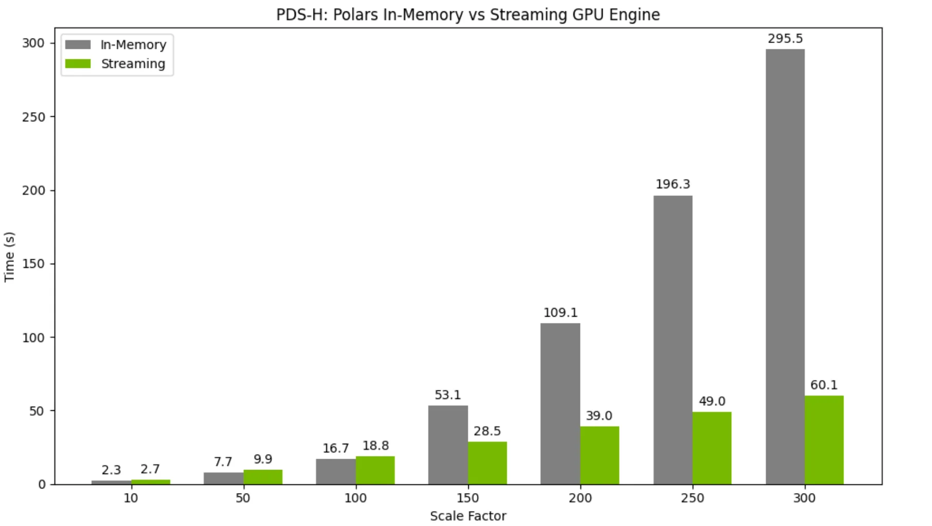
Mode eksekusi streaming yang diperkenalkan sebagai fitur eksperimental di 25.06 sekarang merupakan default di mesin GPU POLAR. Eksekutor baru ini mengambil keuntungan dari partisi data untuk memungkinkan dataset yang jauh lebih besar dari VRAM (memori GPU) diproses secara efisien. Pelaksana streaming masih dapat kembali ke eksekusi dalam memori untuk setiap operasi yang tidak didukung, tetapi pada rilis 25.08, eksekusi streaming mendukung hampir semua operator yang didukung untuk eksekusi GPU dalam memori. Ini membuka kinerja substansial dan peningkatan skalabilitas.
Untuk set data yang lebih kecil, menggunakan mode eksekusi streaming pada GPU tunggal menimbulkan overhead kinerja yang sangat kecil jika dibandingkan dengan menggunakan mesin dalam memori. Namun, ketika ukuran dataset tumbuh dan mulai melebihi memori GPU, pelaksana streaming memberikan percepatan besar dibandingkan dengan mesin dalam memori.
Untuk informasi lebih lanjut tentang pelaksana streaming GPU Polar, kunjungi dokumentasi kami.
Mesin GPU Polar sekarang mendukung data struct di kolom. Sebelumnya, setiap operasi yang melibatkan struct akan kembali ke eksekusi CPU, tetapi dengan rilis terbaru semua operasi ini sekarang diperkuat GPU untuk peningkatan kinerja:
>>> import polars as pl
... ratings = pl.LazyFrame(
...     {
...         "Movie": ["Cars", "IT", "ET", "Cars", "Up", "IT", "Cars", "ET", "Up", "ET"],
...         "Theatre": ["NE", "ME", "IL", "ND", "NE", "SD", "NE", "IL", "IL", "SD"],
...         "Avg_Rating": [4.5, 4.4, 4.6, 4.3, 4.8, 4.7, 4.7, 4.9, 4.7, 4.6],
...         "Count": [30, 27, 26, 29, 31, 28, 28, 26, 33, 26],
...     }
... )
... ratings.select(pl.col("Theatre").value_counts()).collect(engine=pl.GPUEngine(raise_on_fail=True))
...
shape: (5, 1)
┌───────────┐
│ Theatre     │
│ ---         │
│ struct[2]   │
╞═════════==╡
│ {"NE",3}    │
│ {"ND",1}    │
│ {"ME",1}    │
│ {"SD",2}    │
│ {"IL",3}    │
└───────────┘
Selain itu, mesin GPU POLAR sekarang mendukung serangkaian operator string yang diperluas secara substansial, misalnya:
>>> ldf = pl.LazyFrame({"foo": [1, None, 2]})
>>> ldf.select(pl.col("foo").str.join("-")).collect(engine=gpu_engine)
shape: (1, 1)
┌─────┐
│ foo  │
│ ---  │
│ str  │
╞═════╡
│ 1-2  │
└─────┘
>>> ldf = pl.LazyFrame({
...     "lines": [
...         "I Like\nThose\nOdds",
...         "This is\nThe Way",
...     ]
... })
... ldf.with_columns(
...     pl.col("lines").str.extract(r"(T\w+)", 1).alias("matches"),
... ).collect(engine=pl.GPUEngine(raise_on_fail=True))
...
shape: (2, 2)
┌─────────┬──────┐
│ lines   ┆ matches │
│ ---     ┆ ---     │
│ str     ┆ str     │
╞═════════╪══════╡
│ I Like  ┆ Those   │
│ Those   ┆         │
│ Odds    ┆         │
│ This is ┆ This    │
│ The Way ┆         │
└─────────┴──────┘
Perluasan dukungan tipe data semakin memperkuat kemampuan mesin GPU POLAR, mempercepat pengiriman fungsionalitas pengguna akhir yang paling umum.
Dengan rilis 25.08, CUML telah menambahkan algoritma embedding spektral untuk pengurangan dimensi dan pembelajaran berlipat ganda. Embedding spektral adalah pendekatan yang menggunakan nilai eigen dan vektor eigen dari grafik kesamaan untuk menanamkan data dimensi tinggi ke dalam ruang dimensi yang lebih rendah.
API untuk algoritma embedding spektral baru dalam CUML cocok dengan implementasi embedding spektral di scikit-learn:
from cuml.manifold import SpectralEmbedding
import cupy as cp
from sklearn.datasets import fetch_openml


# (70000, 784) -> (70000, 2)
mnist = fetch_openml('mnist_784', version=1)
X, y = mnist.data, mnist.target.astype(int)


spectral = SpectralEmbedding(n_components=2, n_neighbors=None, random_state=42)
embedding = spectral.fit_transform(cp.asarray(X, order='C', dtype=cp.float32))
Selain itu, CUML.Accel sekarang mempercepat beberapa algoritma baru dengan perubahan kode nol. LinearSVC dan LinearSVR Estimator ditambahkan dalam rilis 25.08, yang berarti bahwa semua estimator dalam keluarga mesin vektor dukungan sekarang menjadi bagian dari CUML.Accel.
Kernelridge juga ditambahkan ke CUML.Accel, membawa algoritma regresi populer lainnya di bawah payung perubahan kode nol.
Untuk informasi lebih lanjut tentang algoritma yang didukung hari ini, lihat dokumentasi lengkap kami.
Dimulai dengan rilis 25.08, kami menjatuhkan dukungan untuk CUDA 11, yang mencakup semua kontainer, paket yang diterbitkan, dan kemampuan untuk membangun dari sumber. Pengguna yang ingin terus menjalankan CUDA 11 Mei Pin ke Rapids versi 25.06.
Kunjungi dokumentasi Rapids untuk mempelajari lebih lanjut.
Rilis Nvidia Rapids 25.08 menawarkan lompatan ke depan dalam mempercepat dan mengoptimalkan alur kerja ilmu data. Dengan diperkenalkannya CUML.Accel Profiler, pengembang sekarang memiliki alat yang kuat untuk mendiagnosis dan meningkatkan kinerja kode pembelajaran mesin mereka. Pembaruan untuk mesin GPU POLAR seperti pelaksana streaming dan dukungan tipe data yang diperluas memungkinkan pemrosesan yang efisien dari set data yang besar, meningkatkan skalabilitas dan kinerja. Selain itu, dimasukkannya algoritma baru dalam CUML lebih lanjut merampingkan ekosistem pembelajaran mesin. Perkembangan ini secara kolektif berkontribusi untuk membuat ilmu data yang dipercepat lebih mudah diakses dan efisien bagi pengguna. Untuk menyelam lebih dalam ke semua fitur dan peningkatan baru, pastikan untuk mengunjungi dokumentasi Rapids.
Kami menyambut umpan balik Anda di GitHub. Anda juga dapat bergabung dengan 3.500 anggota komunitas Rapids Slack untuk berbicara pemrosesan data yang dipercepat GPU.
Jika Anda baru mengenal Rapids, periksa sumber daya ini untuk memulai dan mengambil alur kerja Ilmu Data Akselerasi kami dengan Nol Kode Perubahan Kursus secara gratis. Untuk mempelajari lebih lanjut tentang ilmu data yang dipercepat, jelajahi jalur pembelajaran DLI kami dan mendaftar dalam kursus langsung, seperti praktik terbaik dalam rekayasa fitur untuk data tabel dengan akselerasi GPU.